$xlog
[1] FALSE

$ylog
[1] FALSE

$adj
[1] 0.5

$ann
[1] TRUE

$ask
[1] FALSE

$bg
[1] "white"

$bty
[1] "o"

$cex
[1] 1

$cex.axis
[1] 1

$cex.lab
[1] 1

$cex.main
[1] 1.2

$cex.sub
[1] 1

$cin
[1] 0.15 0.20

$col
[1] "black"

$col.axis
[1] "black"

$col.lab
[1] "black"

$col.main
[1] "black"

$col.sub
[1] "black"

$cra
[1] 28.8 38.4

$crt
[1] 0

$csi
[1] 0.2

$cxy
[1] 0.01712329 0.06329115

$din
[1] 9.999999 4.999999

$err
[1] 0

$family
[1] ""

$fg
[1] "black"

$fig
[1] 0 1 0 1

$fin
[1] 9.999999 4.999999

$font
[1] 1

$font.axis
[1] 1

$font.lab
[1] 1

$font.main
[1] 2

$font.sub
[1] 1

$lab
[1] 5 5 7

$las
[1] 0

$lend
[1] "round"

$lheight
[1] 1

$ljoin
[1] "round"

$lmitre
[1] 10

$lty
[1] "solid"

$lwd
[1] 1

$mai
[1] 1.02 0.82 0.82 0.42

$mar
[1] 5.1 4.1 4.1 2.1

$mex
[1] 1

$mfcol
[1] 1 1

$mfg
[1] 1 1 1 1

$mfrow
[1] 1 1

$mgp
[1] 3 1 0

$mkh
[1] 0.001

$new
[1] FALSE

$oma
[1] 0 0 0 0

$omd
[1] 0 1 0 1

$omi
[1] 0 0 0 0

$page
[1] TRUE

$pch
[1] 1

$pin
[1] 8.759999 3.159999

$plt
[1] 0.082 0.958 0.204 0.836

$ps
[1] 12

$pty
[1] "m"

$smo
[1] 1

$srt
[1] 0

$tck
[1] NA

$tcl
[1] -0.5

$usr
[1] 0 1 0 1

$xaxp
[1] 0 1 5

$xaxs
[1] "r"

$xaxt
[1] "s"

$xpd
[1] FALSE

$yaxp
[1] 0 1 5

$yaxs
[1] "r"

$yaxt
[1] "s"

$ylbias
[1] 0.2Lecture 12: Multiple Views
2026-03-05
Multiple Views
The beginning of this lecture is based on Chapter 12 of Visualization Analysis & Design.
“Facet into Multiple Views”
For this lecture, I’m going to start with some principles from the VAD Text, then transition over to creating multi-panel figures in R.
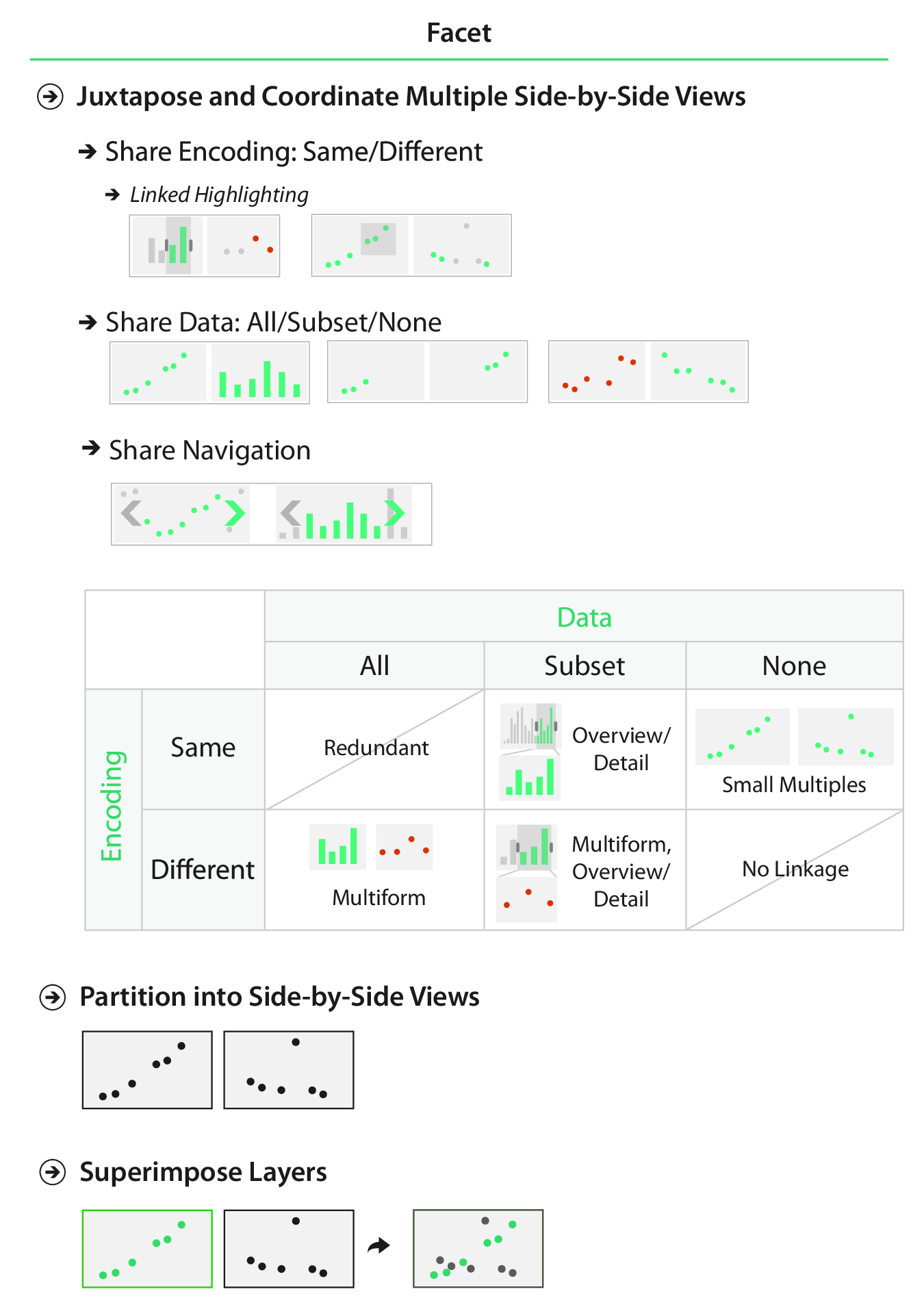
Facet into Multiple Views
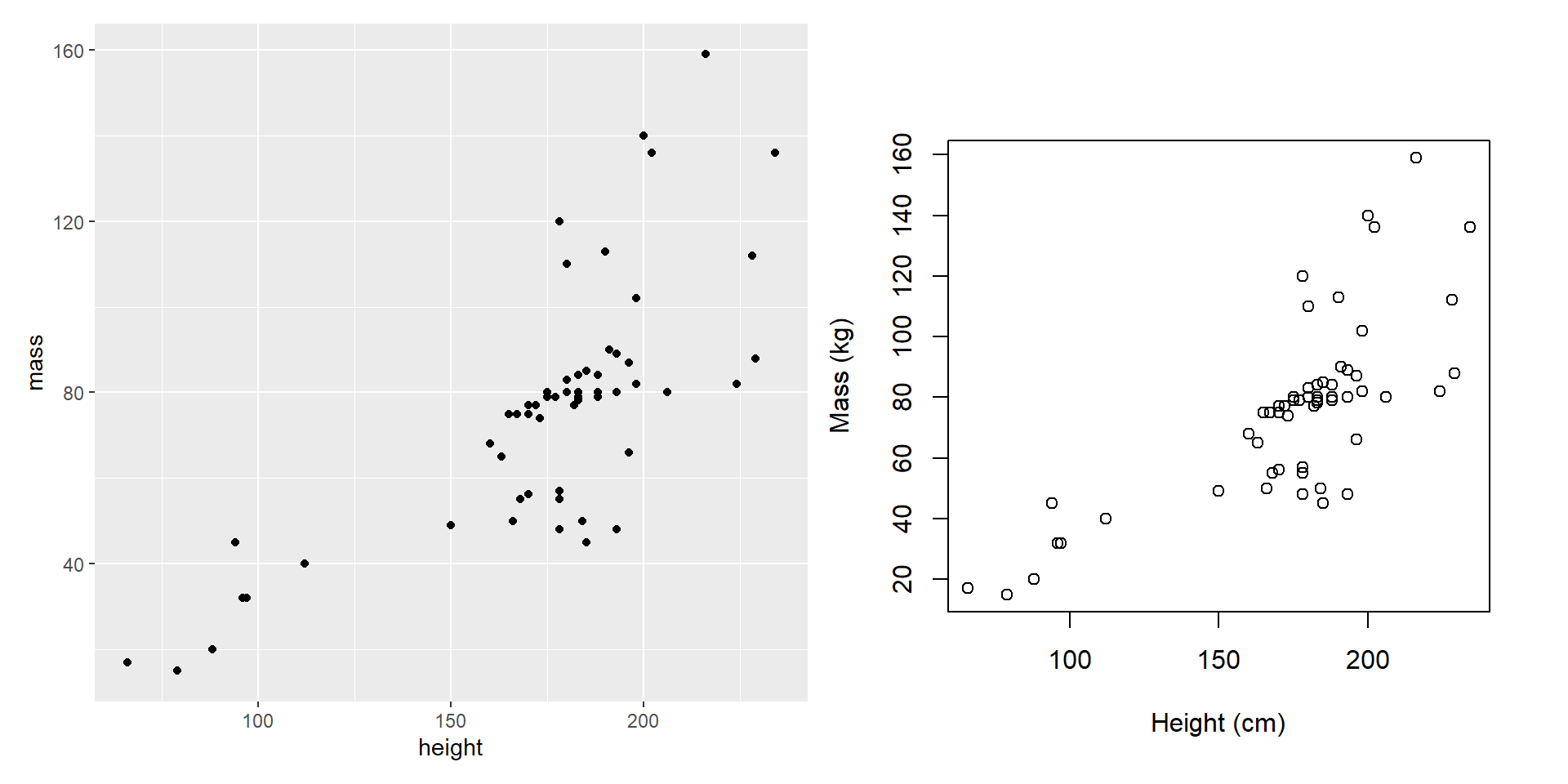
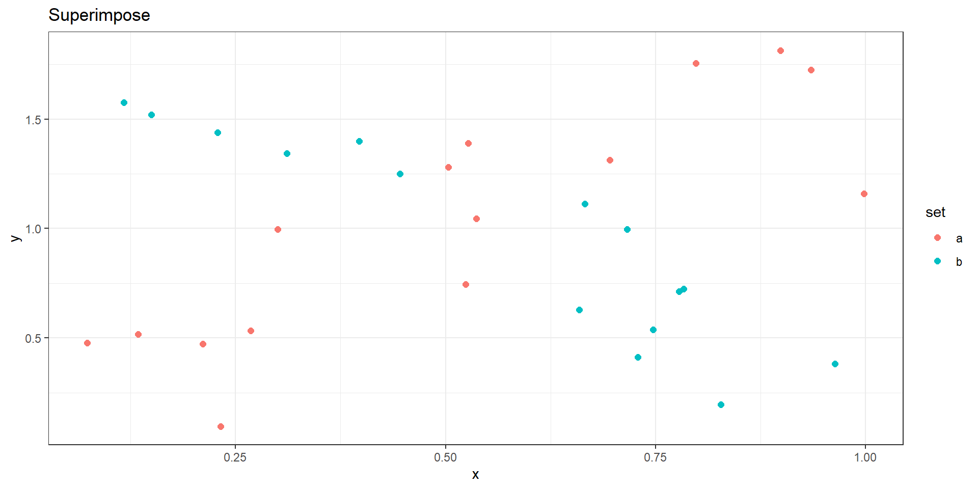
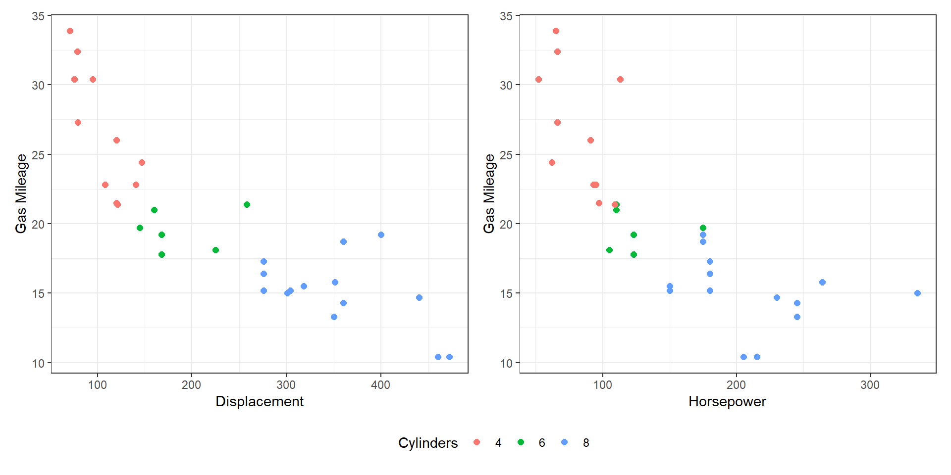
Juxtapose or Superimpose?
Juxtapose or Superimpose?
Share Encoding?
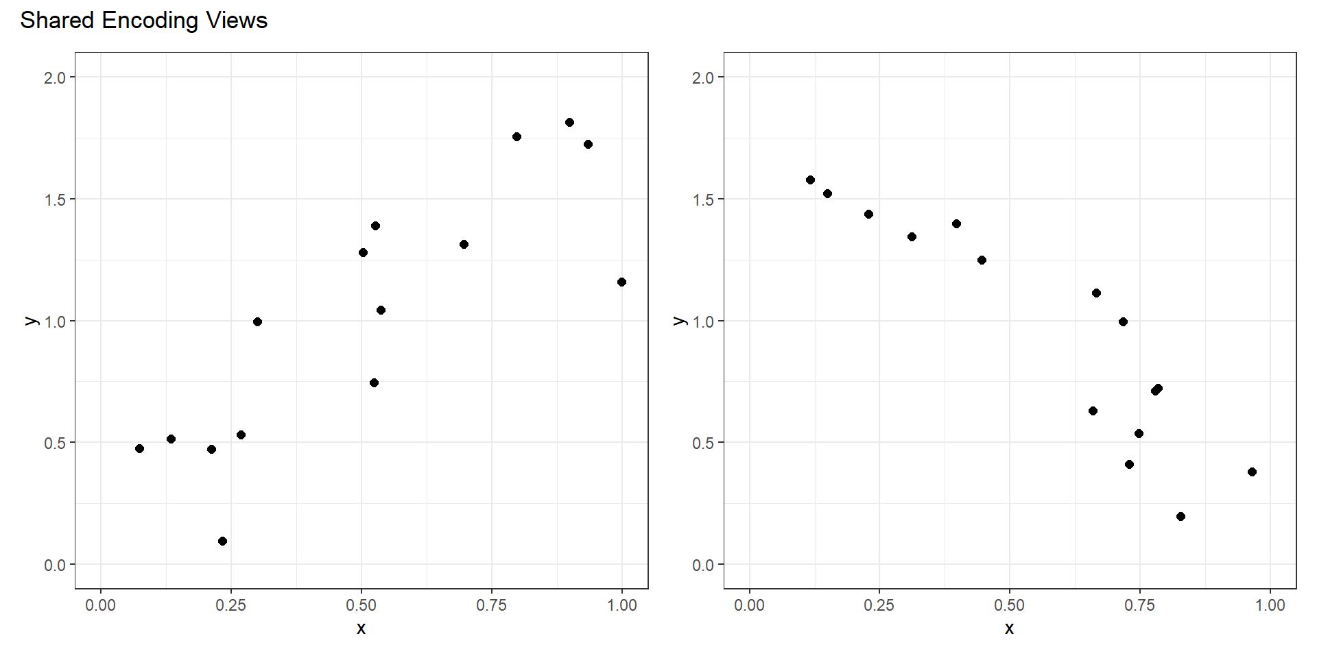
Share Encoding?
Share Encoding?
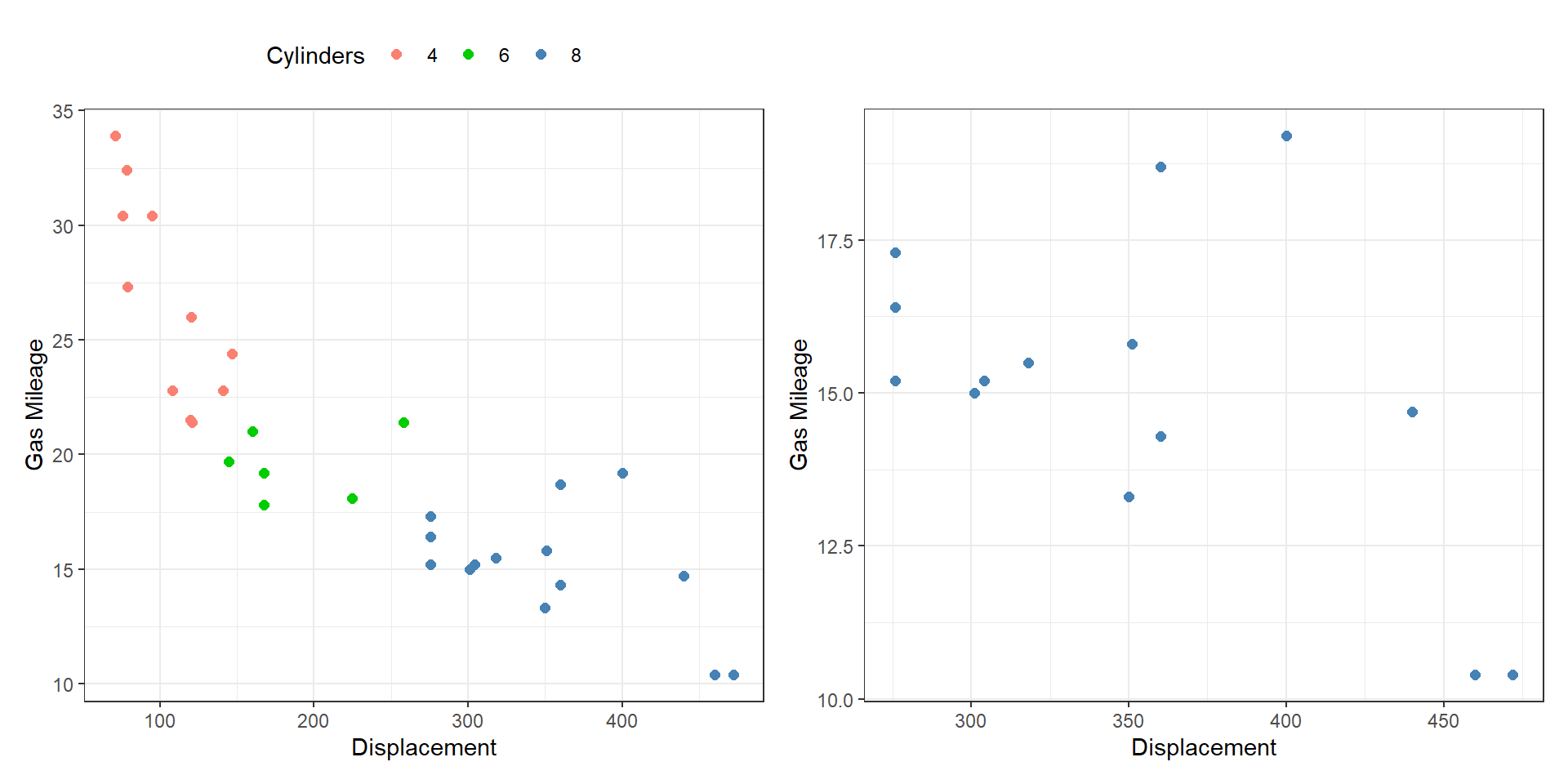
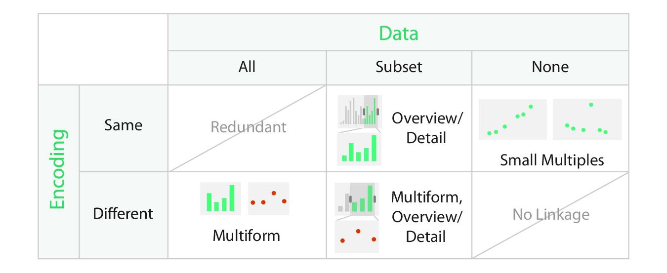
Share Data?
- Shared data (all): both views show all the data.
Share Data?
- Overview-detail (some): one view shows all the data, the other shows detail.
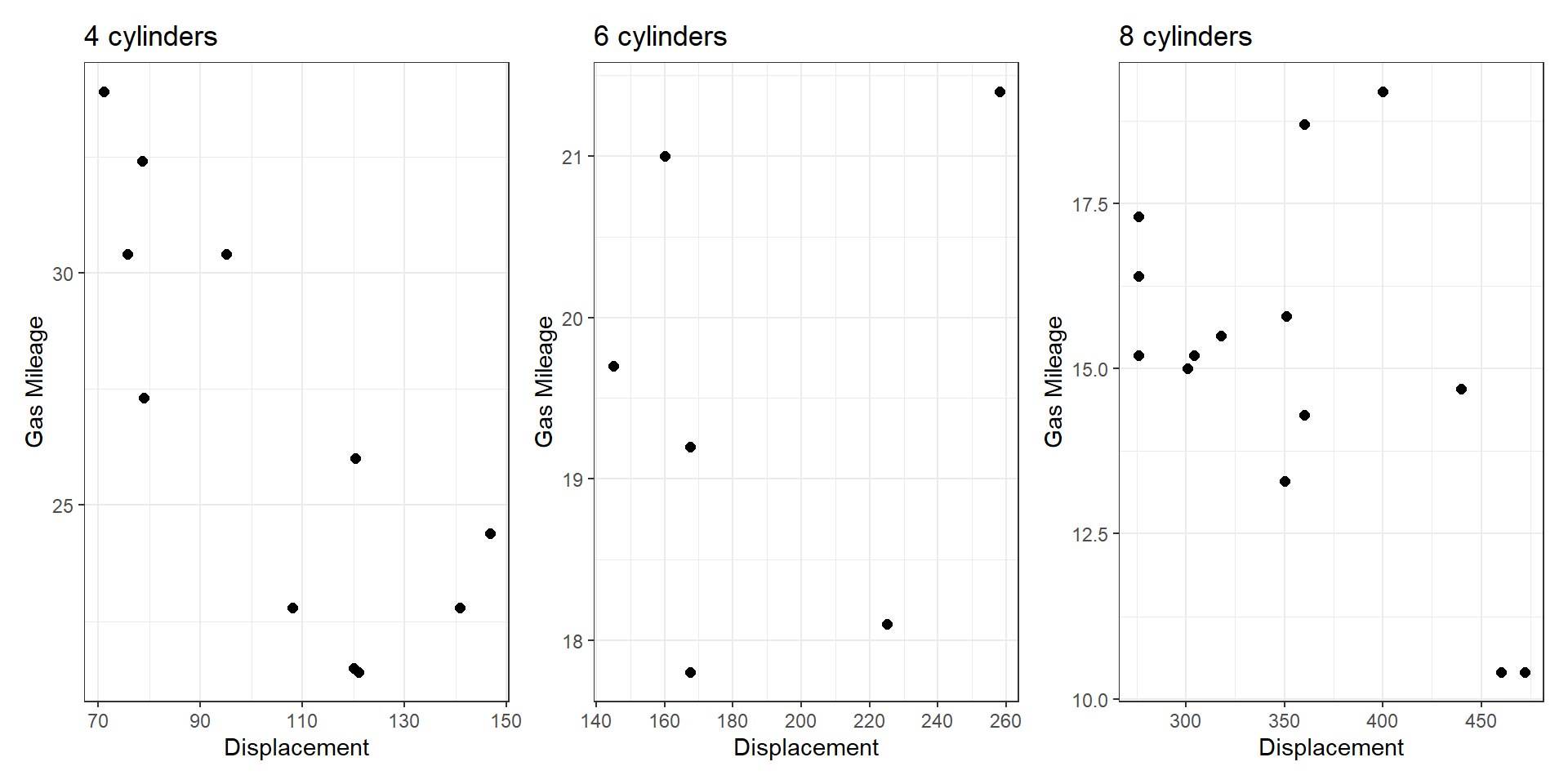
Share Data?
- Small multiples (none): one view shows one subset, the other shows a different subset.
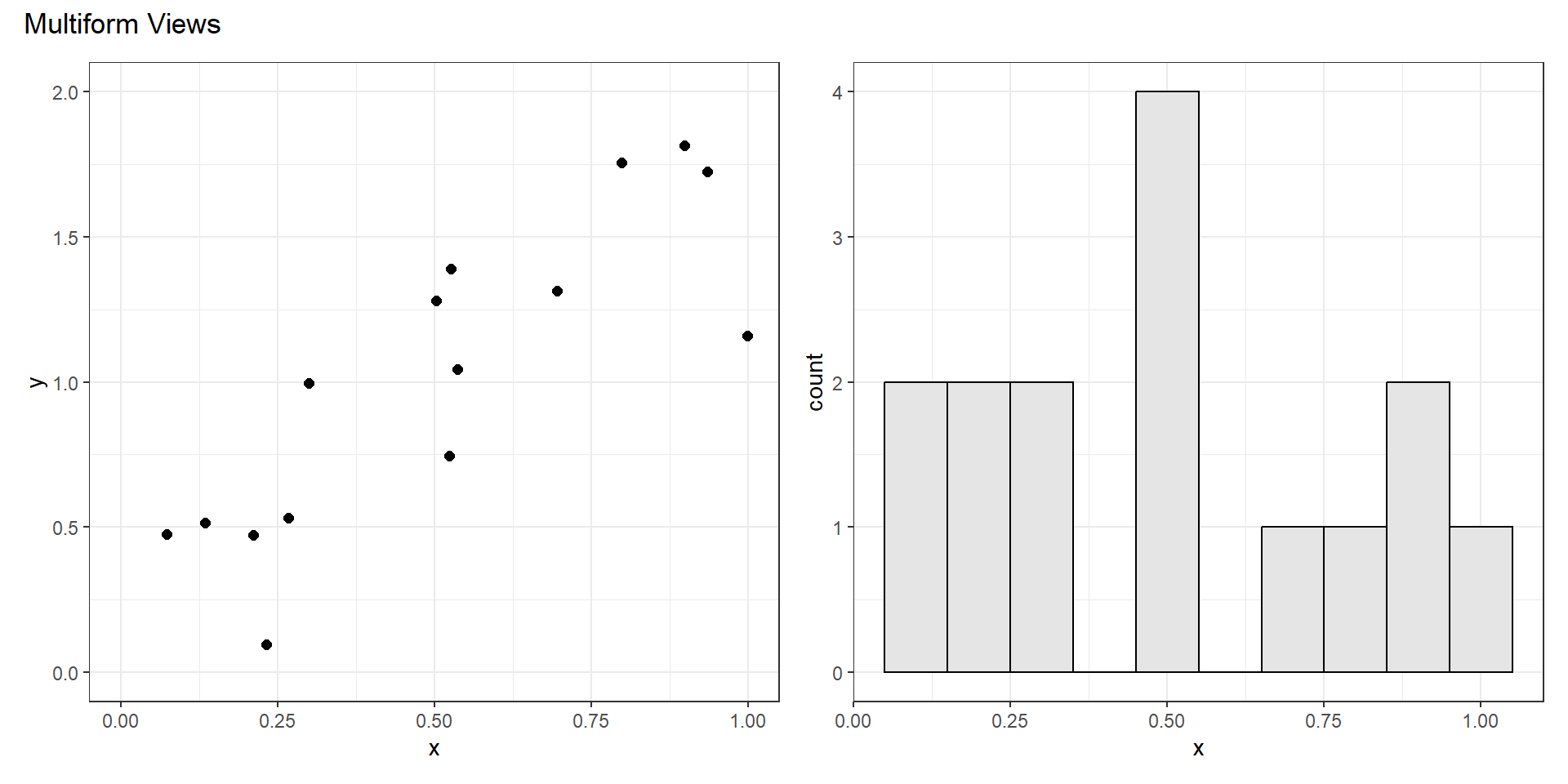
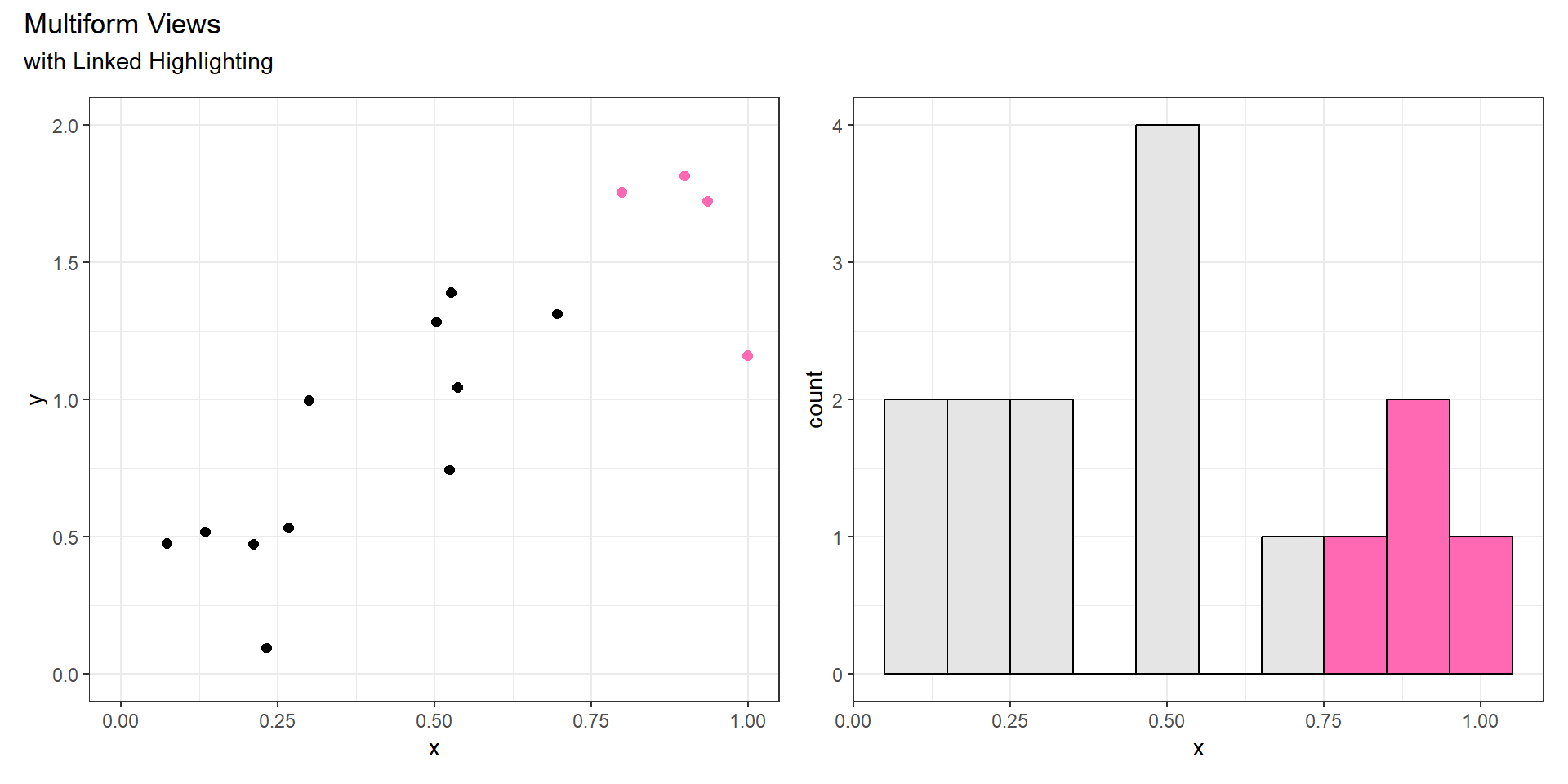
Share Encoding/Data?
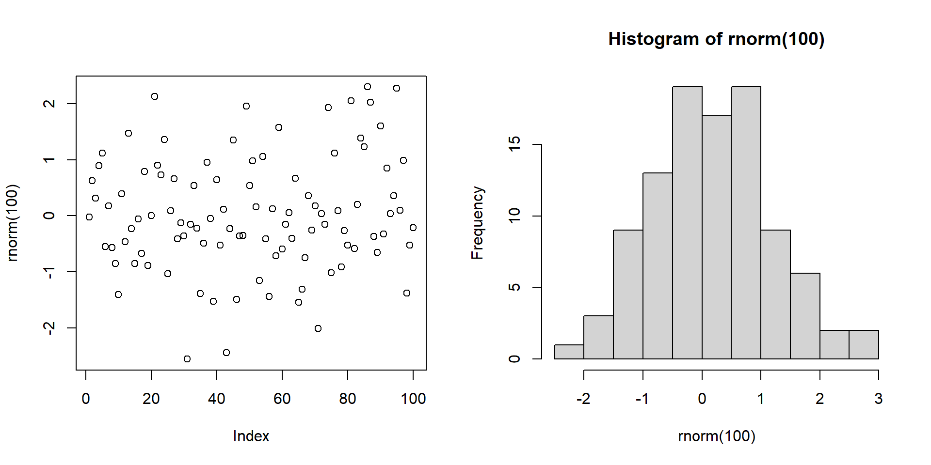
Multi-panel: base R par()
- To create a multi-panel figure, change the graphical parameters
mfrowormfcol.- Specifies the number of rows and columns in the display:
c(nr, nc) - Multiple calls to
plot()are drawn in subsequent rows/columnsmfrowcauses the plots to be drawn by rowsmfcolcauses the plots to be drawn by columns
- Specifies the number of rows and columns in the display:
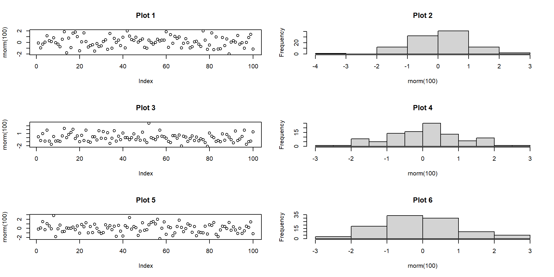
Multi-panel: base R par()
- Use of
mfrow
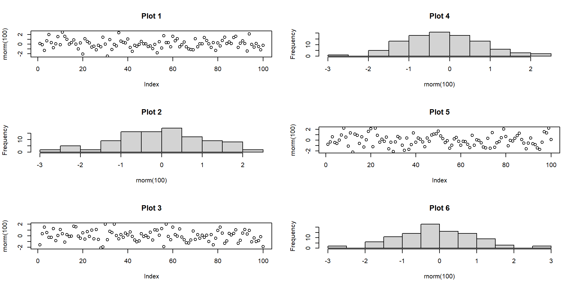
Multi-panel: base R par()
- Use of
mfcol
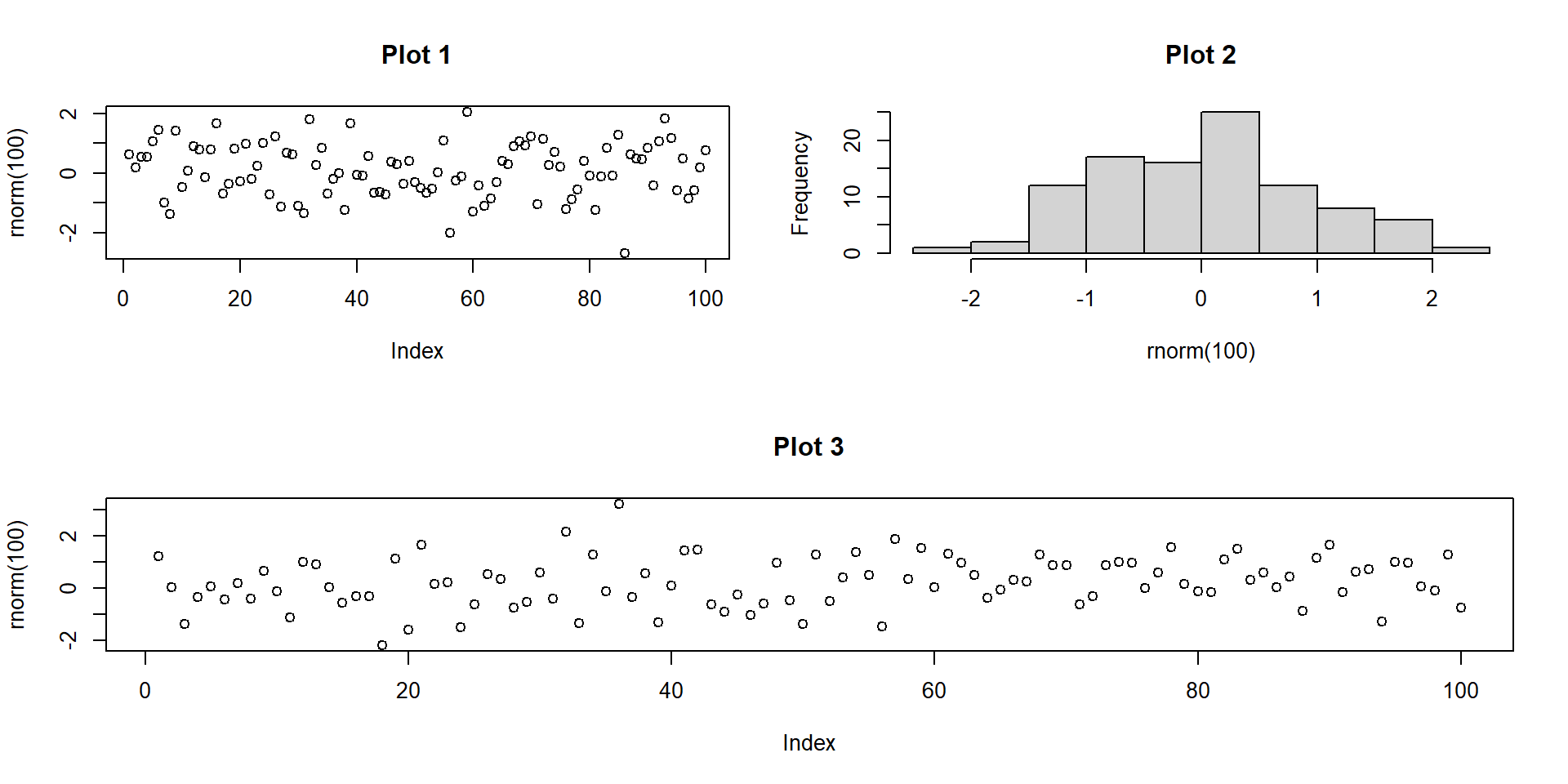
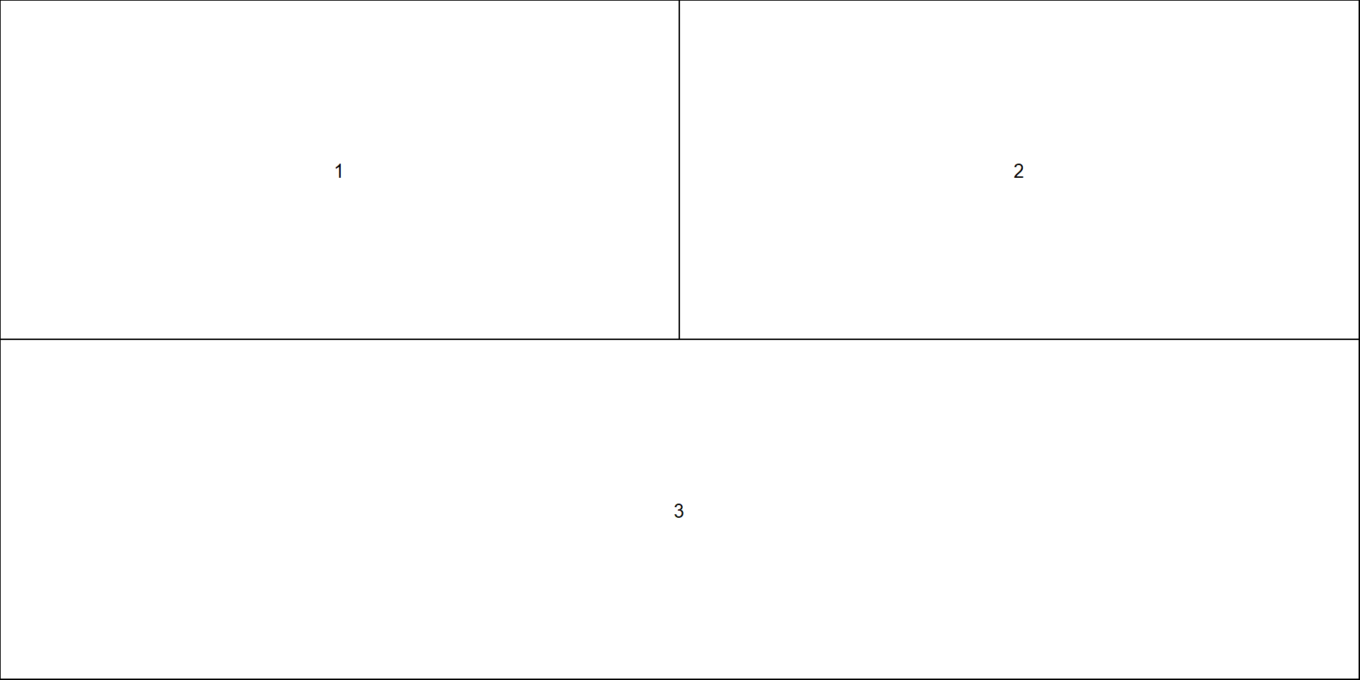
Multi-panel: base R layout()
- Using
layout()allows finer control over the layout using a matrix.- For example, you can allow a single plot to take up multiple slots.
Multi-panel: base R layout()
- There is also function
layout.show()which will show the current layout for planning something complex.
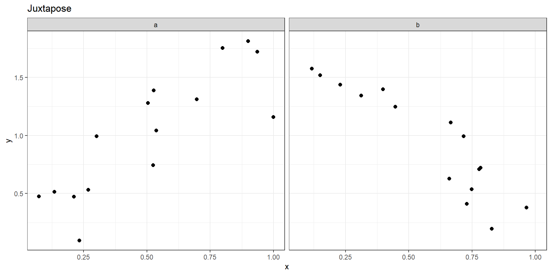
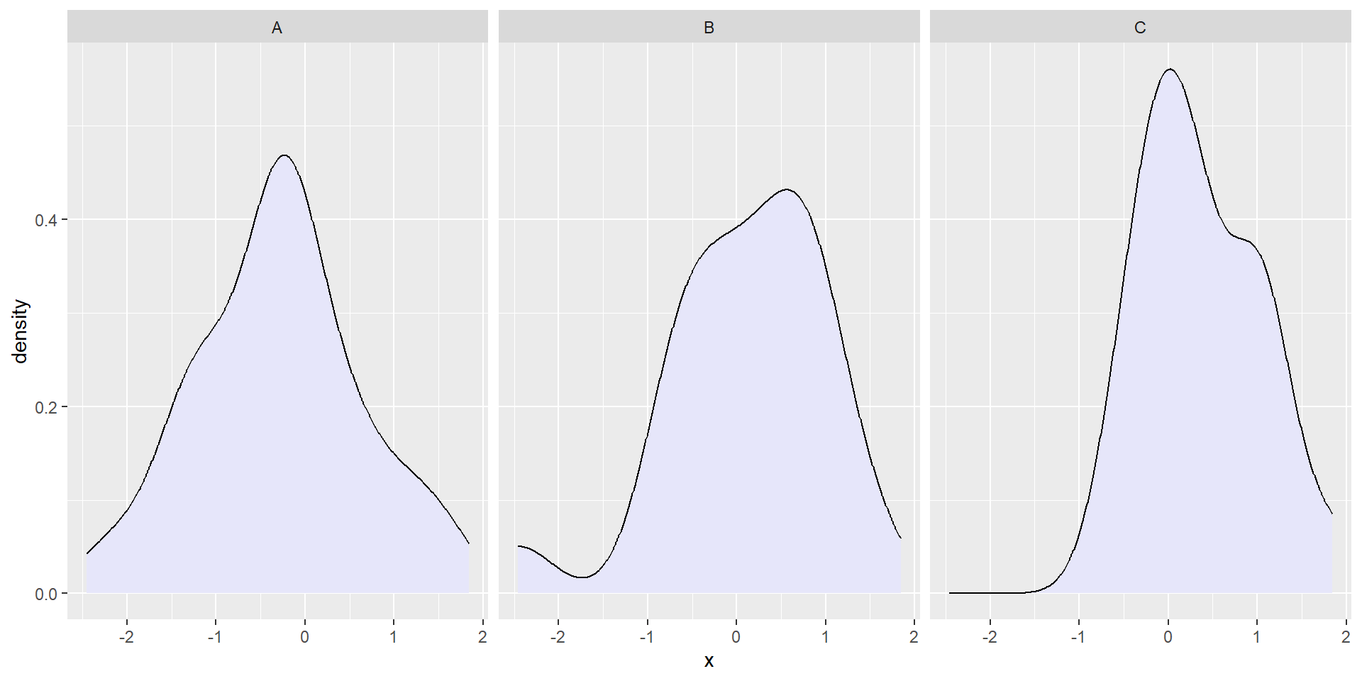
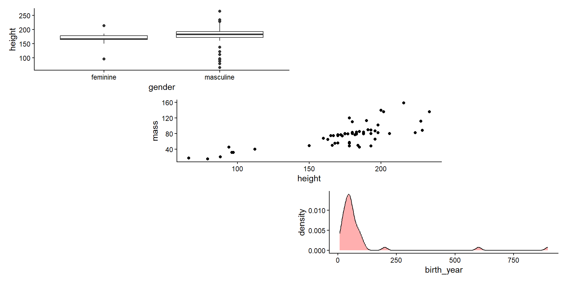
Faceting with ggplot2
facet_wrap()wraps a 1D sequence of panels to fit in the window.
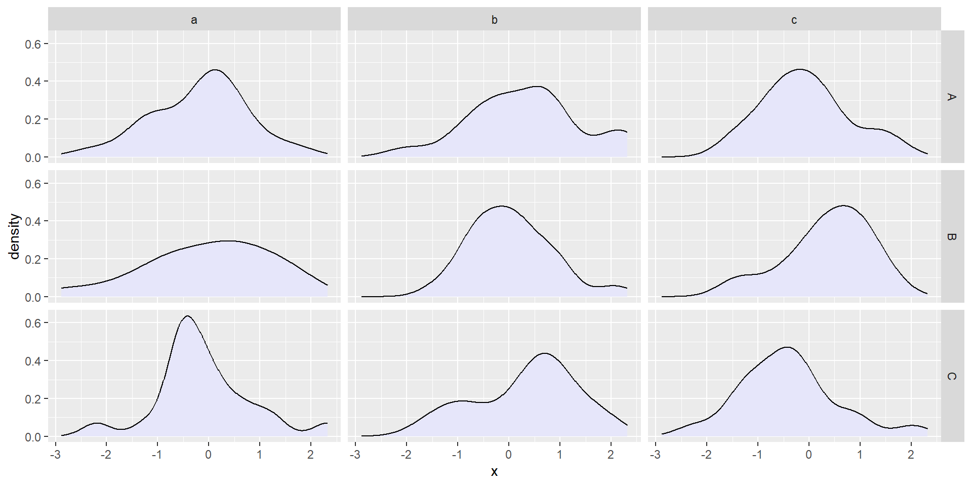
Faceting with ggplot2
facet_grid()forms a matrix of panels defined by rows and columns.
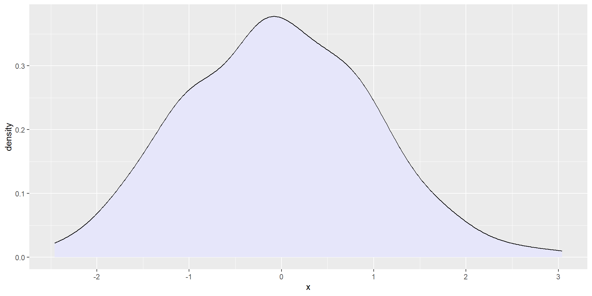
Faceting with ggplot2
facet_null()means no faceting, and can be used to override one of the others.
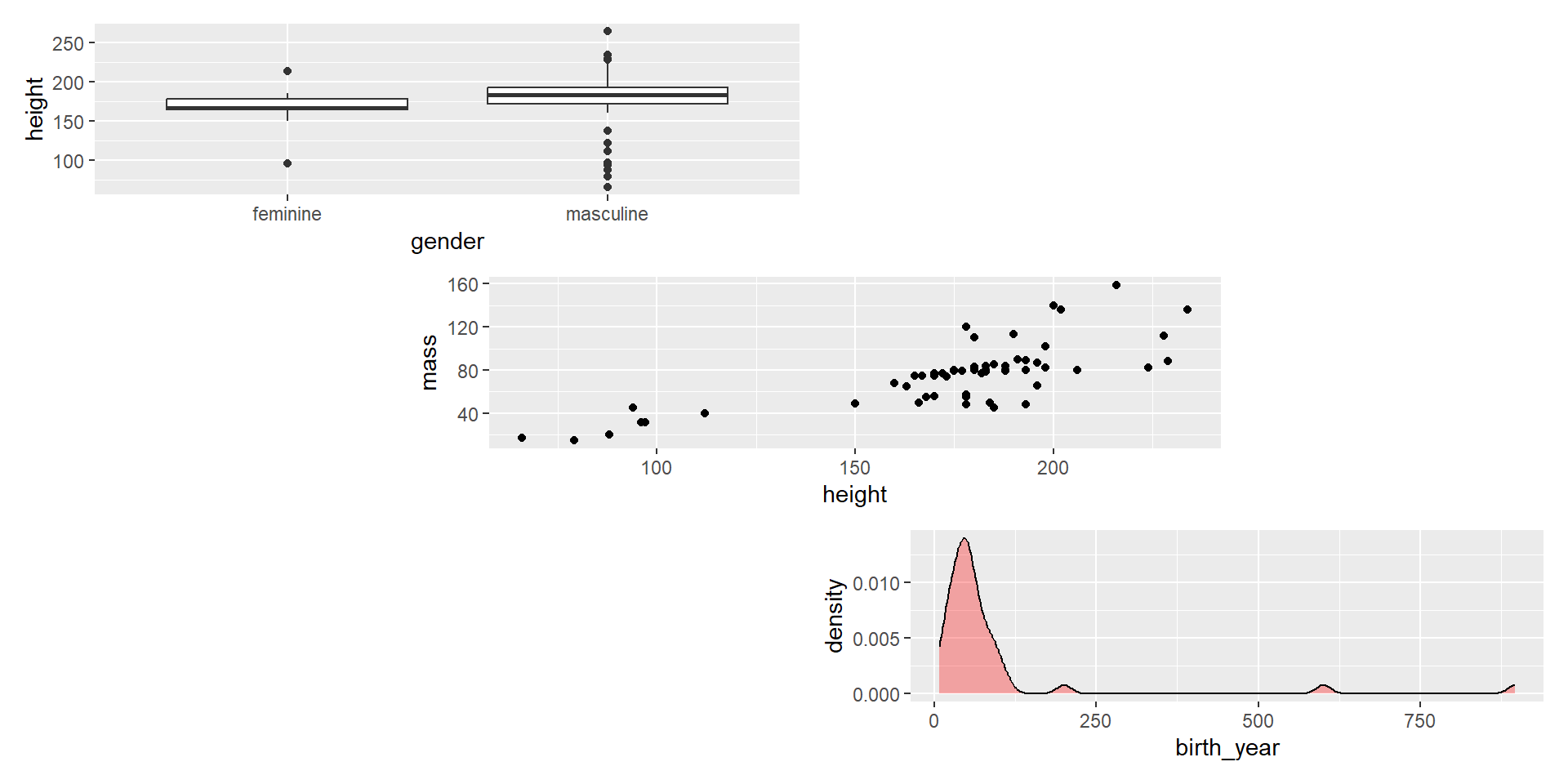
Composing with patchwork
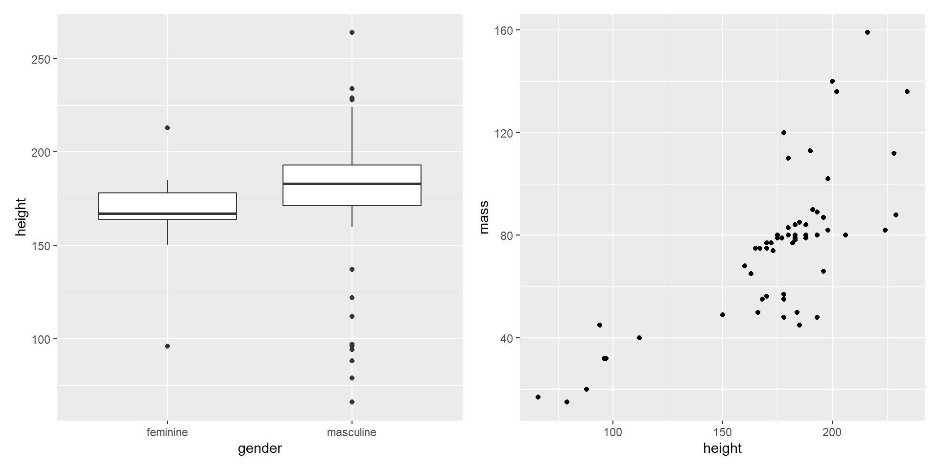
- Combine in a row with
+
Composing with patchwork
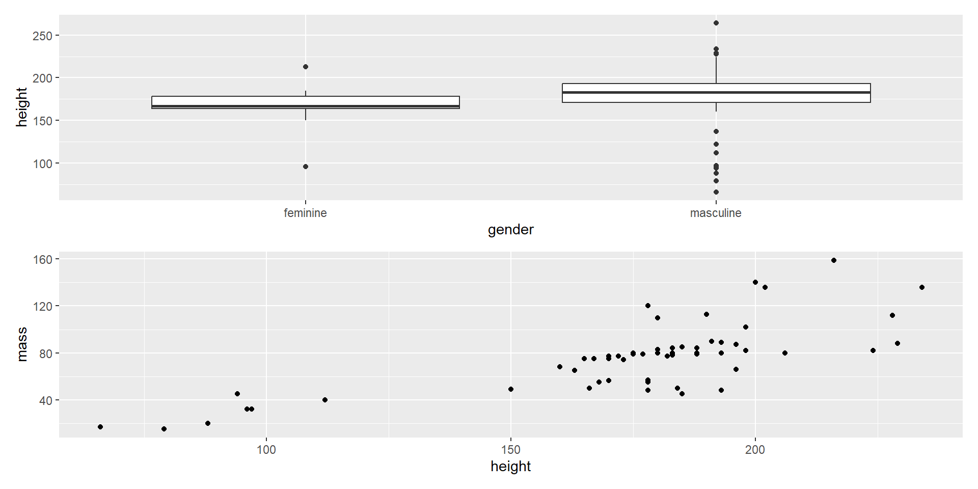
- Combine in a column with
/
Composing with patchwork
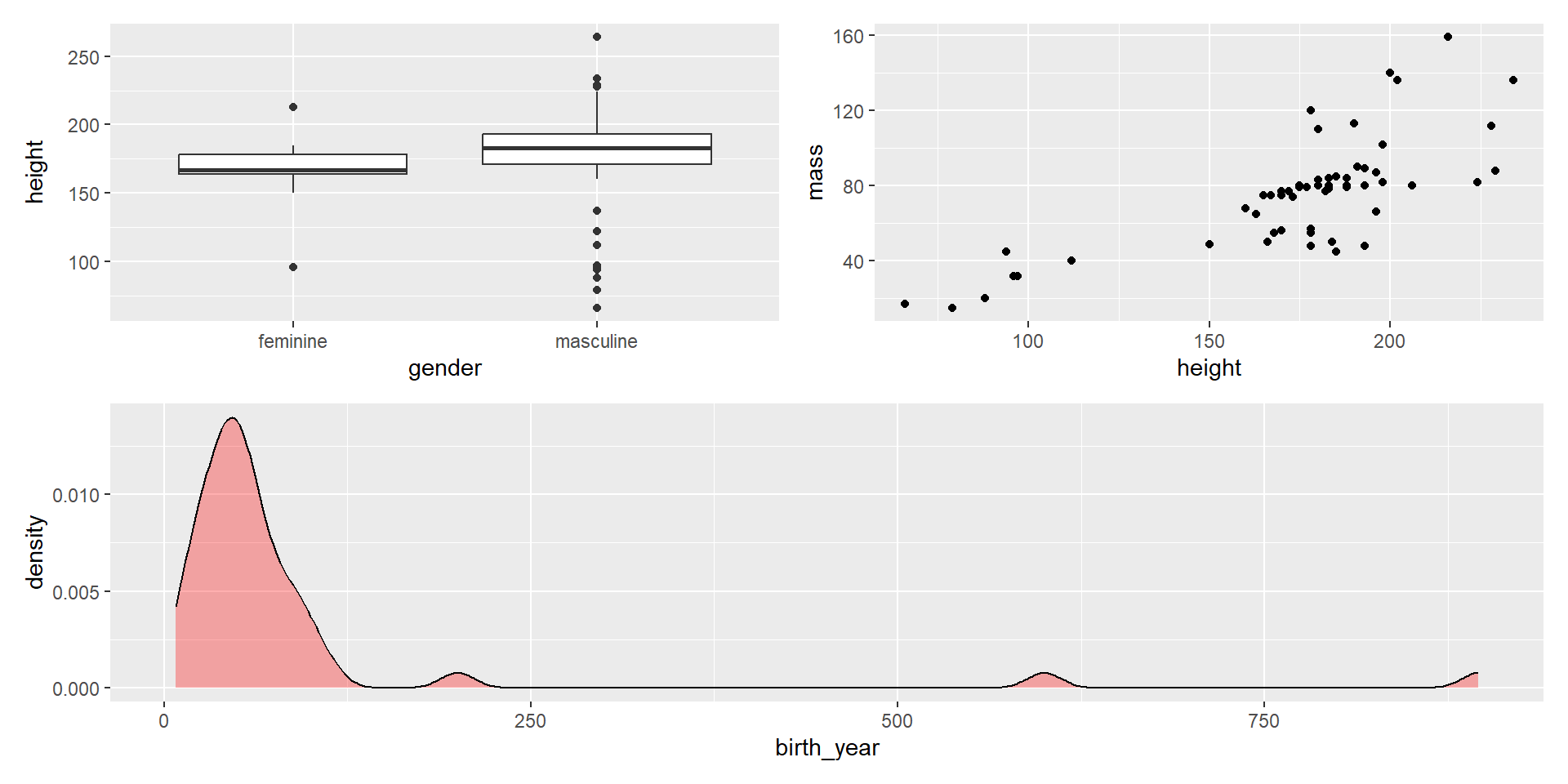
- Group plots to increase complexity with
()
Composing with patchwork
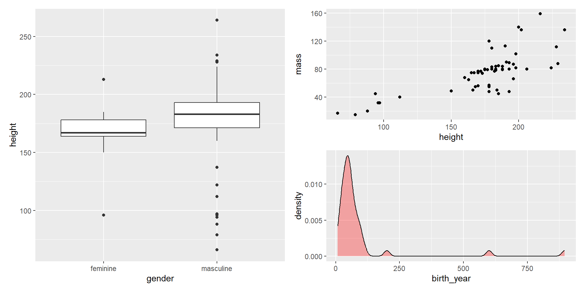
- Group plots to increase complexity with
()
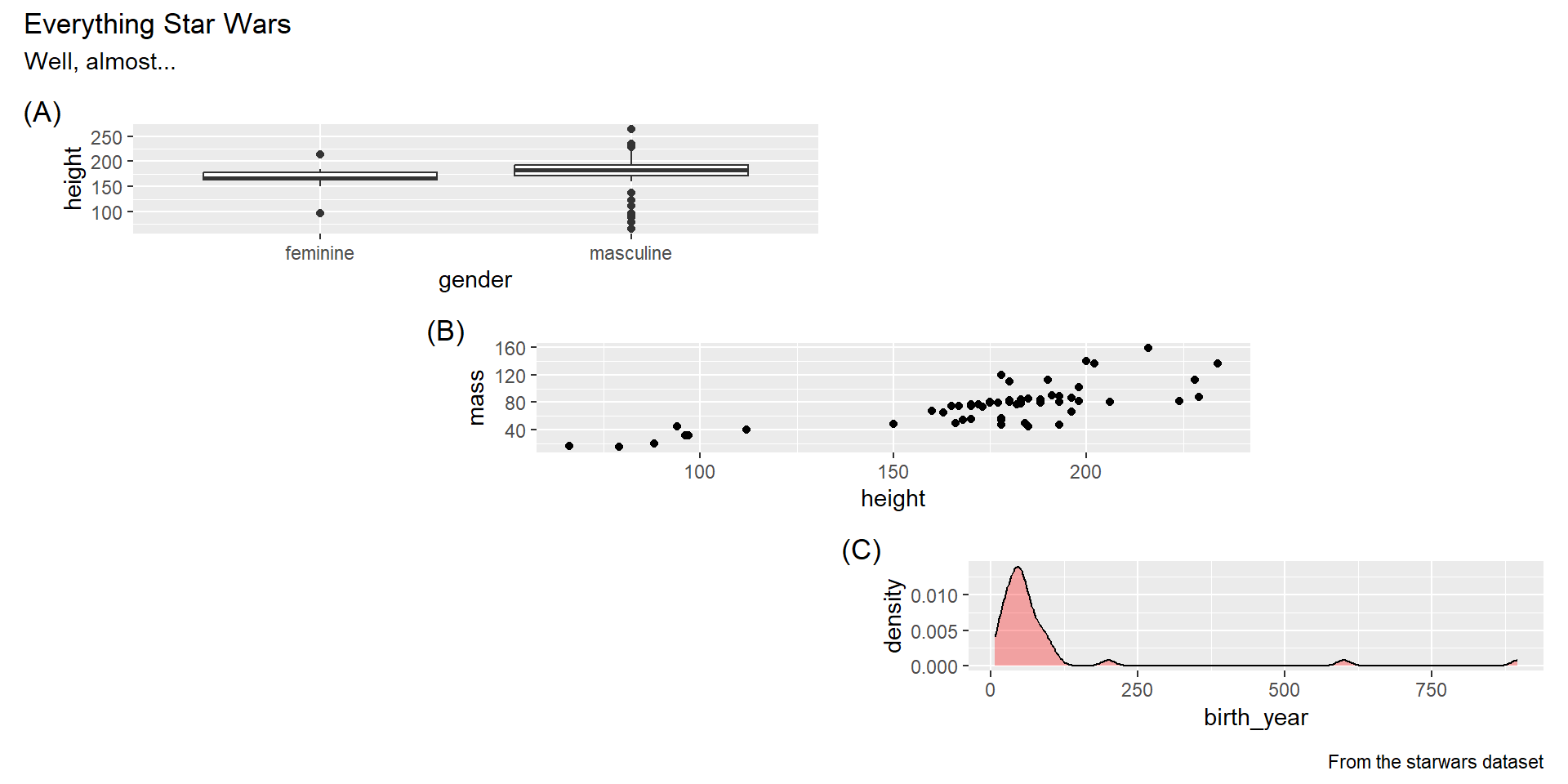
Composing with patchwork
- For more fine-scale control (and options), use
plot_layout().
Composing with patchwork
- Add annotations with
plot_annotation().
Composing with patchwork
- You can still add to existing plots…
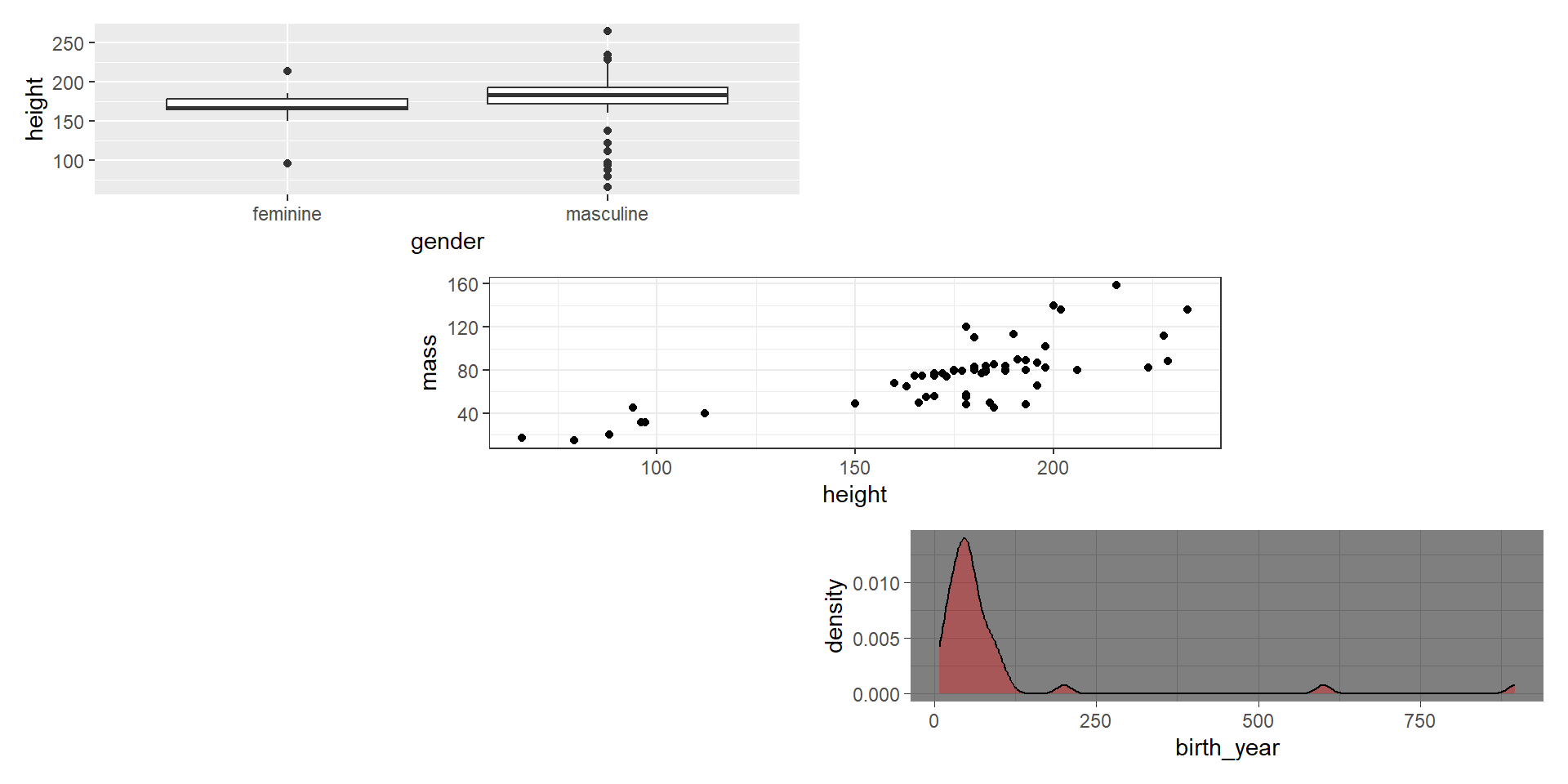
Composing with patchwork
- … but you can change the theme of all plots with
&.
Composing with patchwork
- Plots with legends will show the legend.
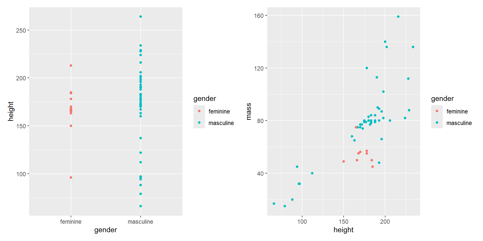
Composing with patchwork
- You can also “collect” all the legends.
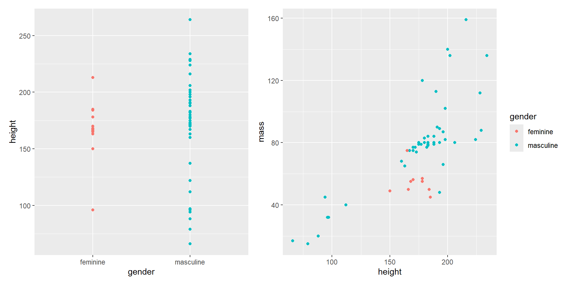
Composing with patchwork
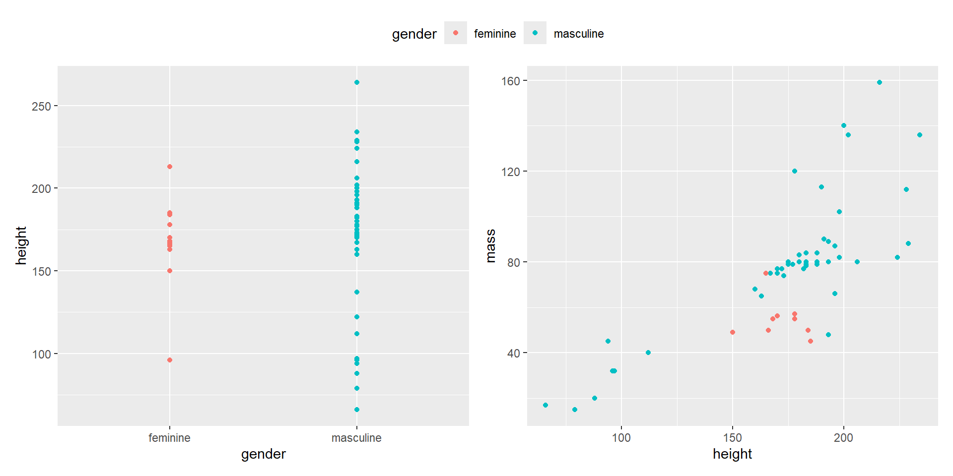
- You can also use
&to change all the legend positions that are being collected.
Composing with patchwork
- You can include base R plots (or other plots) with
wrap_elements().