Lecture 14: Reducing Items and Attributes

Brian J. Smith

2026-03-26

Reducing Items and Attributes

The beginning of this lecture is based on Chapter 13 of Visualization Analysis & Design.

“Reduce Items and Attributes”

For this lecture, I’m going to start with the VAD Text, then transition over to R.

Fig. 13.1

Reducing Items and Attributes

Why?

• Manage complexity in our visualizations.
• Find a strategy that reduces the visual complexity while minimizing the changes of hiding important information from the user.

Reducing Items and Attributes

How?

• Filter:
  • Eliminating elements (items or attributes).
  • Easy to understand and compute.
  • But, “out of sight, out of mind.”
• Aggregate:
  • Creating a new single element to replace multiple others.
  • Challenging to design and convey.
  • Safer cognitively to avoid forgetting filtered information.

Filtering

• Straightfoward and intuitive.
  • Just don’t show some things!
  • Common when exploring a new dataset.
• Plot only some attributes (columns).
  • Often based on knowledge of what the attributes represent.
• Plot only some items (rows).
  • Often based on values.
  • Sometimes based on a random subset.

Filtering

Attribute Filtering

• Often, we have an idea which attributes are most important to us.
  • Prioritize visualizations with those attributes.

data("mtcars")

plot(mtcars)

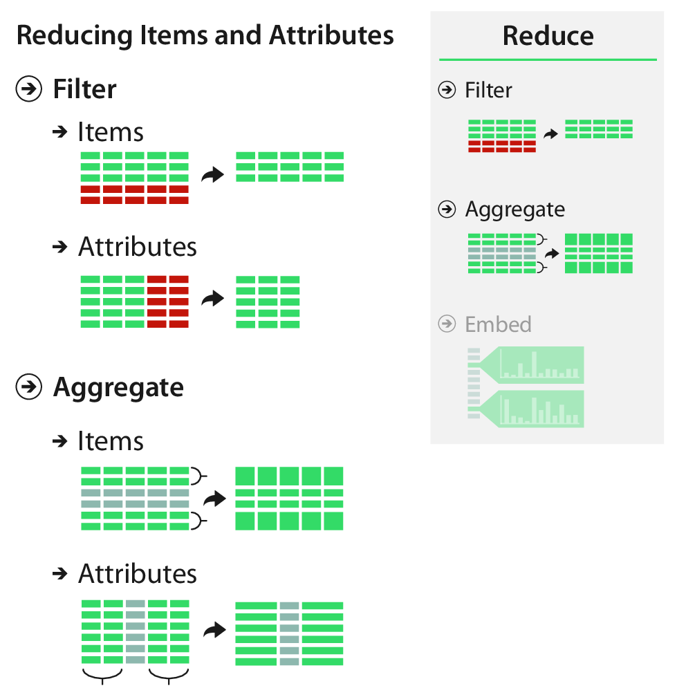
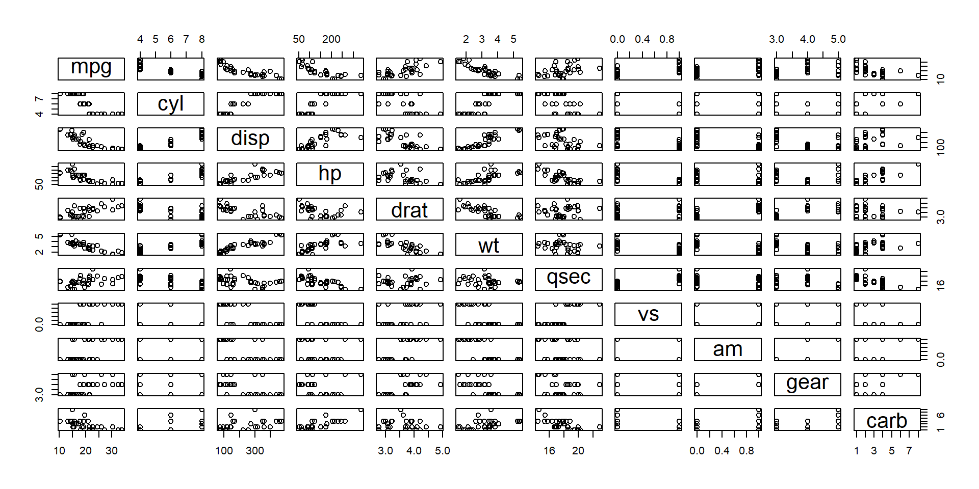
Filtering

Attribute Filtering

• This may be combined with attribute ordering.
  • Orders attributes based on their similarity.
  • E.g., highly correlated attributes show some redundant information.

a <- mtcars %>% 
  ggplot(aes(x = disp, y = hp)) +
  geom_point() +
  geom_label(x = 150, y = 300, 
             label = paste("r =", 
                           round(cor(mtcars$disp, 
                                     mtcars$hp,
                                     method = "spearman"),
                                 2))) +
  geom_smooth(method = "lm", se = FALSE) +
  theme_classic()

b <- mtcars %>% 
  ggplot(aes(x = disp, y = mpg)) +
  geom_point() +
  theme_classic()

c <- mtcars %>% 
  ggplot(aes(x = hp, y = mpg)) +
  geom_point() +
  theme_classic()

des <- "AB
        AC"

a + b + c + plot_layout(widths = c(0.3, 0.7),
                        design = des)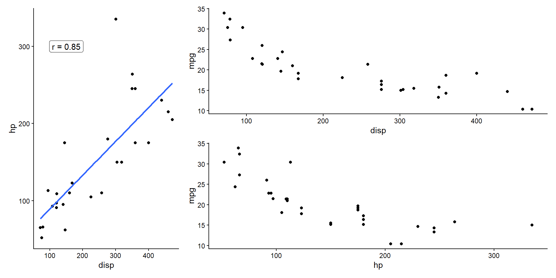

Filtering

Item Filtering

• Filter items based on values.
  • E.g., remove outliers or extreme values.

data("starwars")

a <- starwars %>% 
  ggplot(aes(x = height, y = mass)) +
  geom_point() +
  coord_cartesian(xlim = c(50, 250)) +
  ggtitle("Without Filtering") +
  theme_classic()

b <- starwars %>% 
  filter(mass < 500) %>% 
  ggplot(aes(x = height, y = mass)) +
  geom_point() +
  coord_cartesian(xlim = c(50, 250)) +
  ggtitle("Filter Extreme Values") +
  theme_classic()

a/b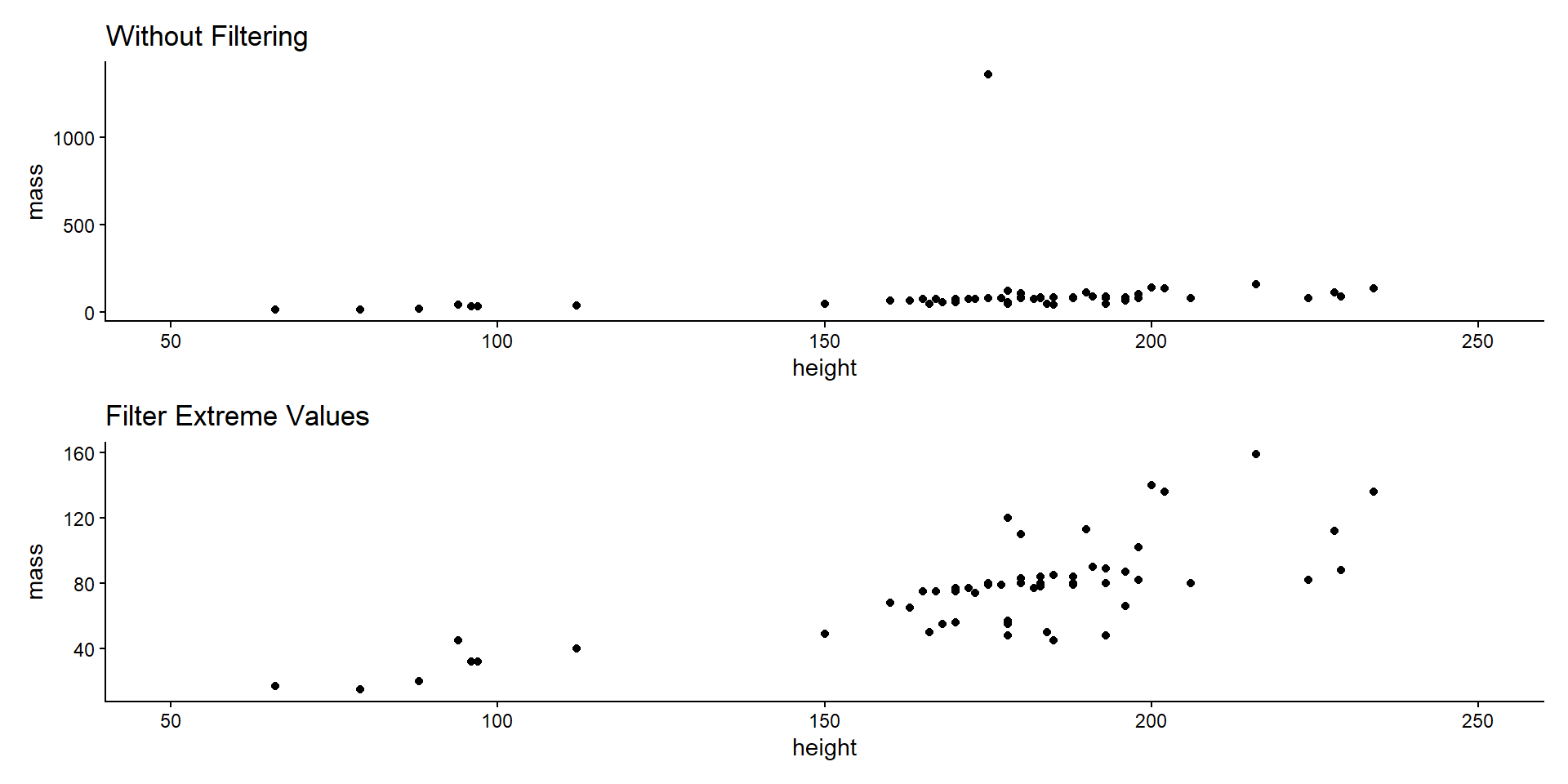

Filtering

Item Filtering

• Randomly subset items.
  • Useful for (truly) big datasets where plotting all items would be difficult (impossible).

# See ?dplyr::slice_sample

# Can specify number of items
mtcars %>% 
  slice_sample(n = 5)

# Can specify proportion of rows
mtcars %>% 
  slice_sample(prop = 0.1)

Aggregation

• Creating a new derived element to represent the group.
  • Simple examples include summary statistics.
  • Remember Anscombe’s Quartet!

Aggregation

Item Aggregation

• Easily accomplished with idioms that:
  • Display summary statistics.
    • Mean, SD, etc. (moments)
    • Counts, densities
  • Show distributions.

Aggregation

Item Aggregation

1D Summary Stats

a <- starwars %>% 
  filter(mass < 500) %>% 
  ggplot(aes(x = 0, y = mass)) +
  geom_point(show.legend = FALSE) +
  ggtitle("Without Aggregation") +
  labs(x = NULL, y = "Mass") +
  theme_classic() +
  theme(axis.text.x = element_text(angle = 45, hjust = 1))

b <- starwars %>%
  filter(mass < 500) %>% 
  ggplot(aes(y = mass)) +
  geom_boxplot(show.legend = FALSE) +
  ggtitle("Aggregate with Summary Stats (Boxplot)") +
  labs(x = NULL, y = "Mass") +
  theme_classic() +
  theme(axis.text.x = element_text(angle = 45, hjust = 1))

a/b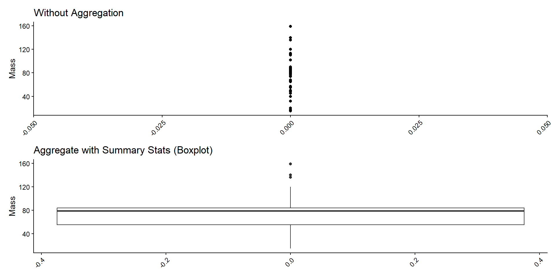

Aggregation

Item Aggregation

2D Summary Stats

spp <- starwars %>% 
  filter(!is.na(species)) %>% 
  count(species) %>% 
  filter(n > 1)

sw <- starwars %>% 
  filter(species %in% spp$species) %>% 
  mutate(species = factor(species))

a <- sw %>% 
  ggplot(aes(x = species, y = mass, color = species)) +
  geom_point(show.legend = FALSE) +
  ggtitle("Without Aggregation") +
  labs(x = "Species", y = "Mass") +
  theme_classic() +
  theme(axis.text.x = element_text(angle = 45, hjust = 1))

b <- sw %>%
  ggplot(aes(x = species, y = mass, 
             color = species)) +
  geom_boxplot(show.legend = FALSE) +
  ggtitle("Aggregate by Species (Boxplot)") +
  labs(x = "Species", y = "Mass") +
  theme_classic() +
  theme(axis.text.x = element_text(angle = 45, hjust = 1))

a/b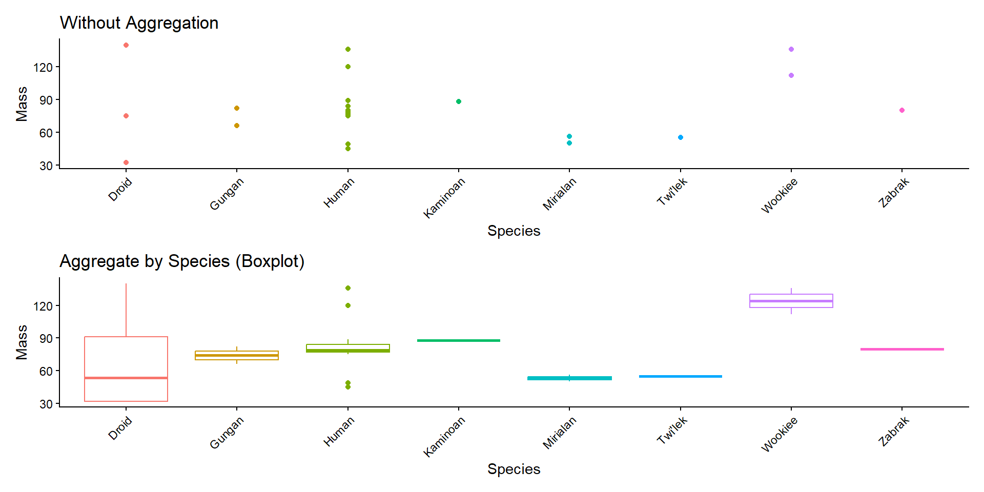

Aggregation

Item Aggregation

3D Summary Stats

# 'sw' created on previous slide

a <- sw %>% 
  ggplot(aes(x = height, y = mass, color = species)) +
  geom_point(show.legend = FALSE) +
  coord_cartesian(xlim = c(50, 250)) +
  ggtitle("Without Aggregation") +
  labs(x = "Height", y = "Mass") +
  theme_classic()

b <- sw %>% 
  group_by(species) %>% 
  summarize(mass_mean = mean(mass, na.rm = TRUE),
            mass_sd = sd(mass, na.rm = TRUE),
            height_mean = mean(height, na.rm = TRUE),
            height_sd = sd(height, na.rm = TRUE)) %>% 
  mutate(mass_lwr = mass_mean - mass_sd,
         mass_upr = mass_mean + mass_sd,
         height_lwr = height_mean - height_sd,
         height_upr = height_mean + height_sd) %>% 
  ggplot(aes(x = height_mean, y = mass_mean, 
             color = species)) +
  geom_errorbar(aes(xmin = height_lwr, xmax = height_upr),
                width = 5) +
  geom_errorbar(aes(ymin = mass_lwr, ymax = mass_upr),
                width = 2) +
  geom_point(size = 2) +
  coord_cartesian(xlim = c(50, 250)) +
  ggtitle("Aggregate by Species (mean +/- SD)") +
  labs(x = "Height", y = "Mass") +
  theme_classic()

a/b + plot_layout(guides = "collect")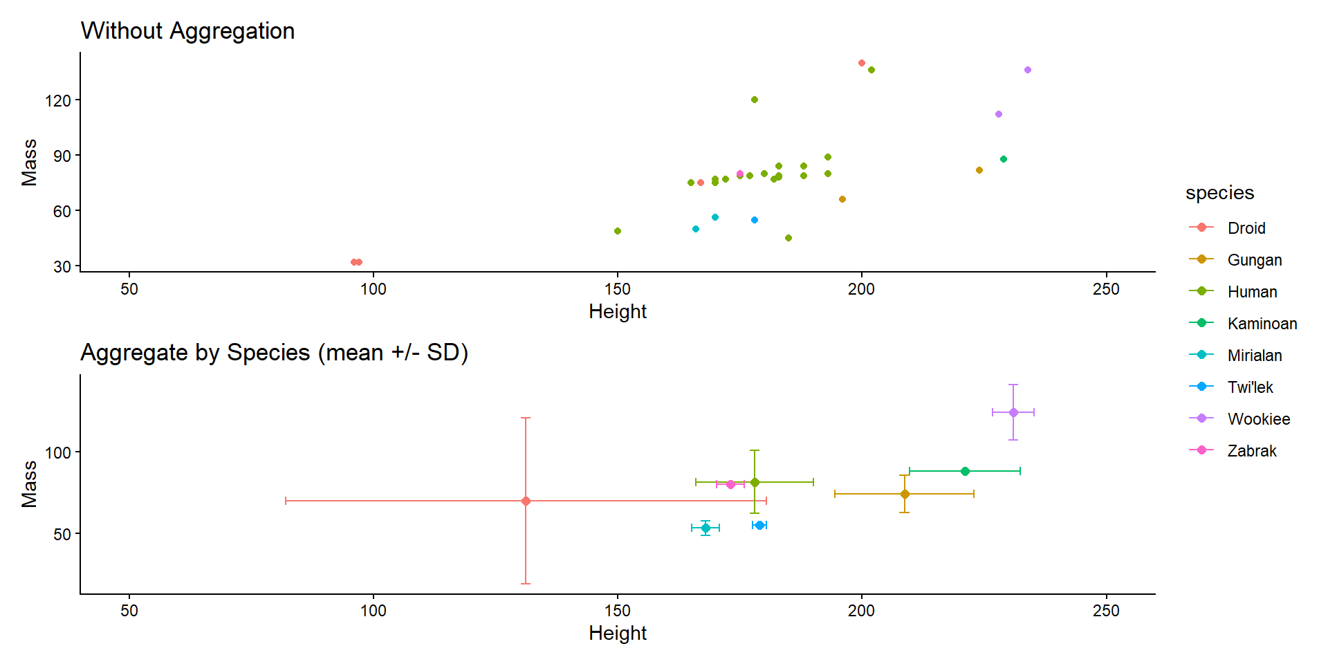

Aggregation

Item Aggregation

1D Counts/Densities

a <- starwars %>% 
  filter(mass < 500) %>% 
  ggplot(aes(y = 0, x = height)) +
  geom_point(show.legend = FALSE) +
  ggtitle("Without Aggregation") +
  labs(x = "Height", y = NULL) +
  theme_classic()

b <- starwars %>%
  filter(mass < 500) %>% 
  ggplot(aes(x = height)) +
  geom_histogram(bins = 15, color = "black", fill = "gray") +
  ggtitle("Aggregate with Counts (Histogram)") +
  labs(x = "Height", y = "Count") +
  theme_classic()

c <- starwars %>%
  filter(mass < 500) %>% 
  ggplot(aes(x = height)) +
  geom_density(color = "black", fill = "gray") +
  ggtitle("Aggregate with Density (KDE)") +
  labs(x = "Height", y = "Density") +
  theme_classic()

a/(b+c)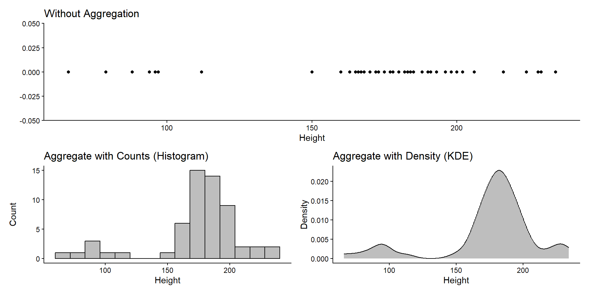

Aggregation

Item Aggregation

2D Summary Stats

# 'sw' created on an earlier slide

a <- sw %>% 
  ggplot(aes(x = species, y = mass, color = species)) +
  geom_point(show.legend = FALSE) +
  ggtitle("Without Aggregation") +
  labs(x = "Species", y = "Mass") +
  theme_classic() +
  theme(axis.text.x = element_text(angle = 45, hjust = 1))

b <- sw %>%
  filter(!is.na(mass)) %>% 
  mutate(mass_bin = cut_number(mass, n = 5)) %>% 
  group_by(species, mass_bin) %>% 
  tally() %>% 
  ggplot(aes(x = species, y = mass_bin, 
             fill = n)) +
  geom_raster() +
  ggtitle("Aggregate with Counts (Heatmap)") +
  labs(x = "Species", y = "Mass") +
  scale_fill_viridis_c() +
  theme_classic() +
  theme(axis.text.x = element_text(angle = 45, hjust = 1))

a/b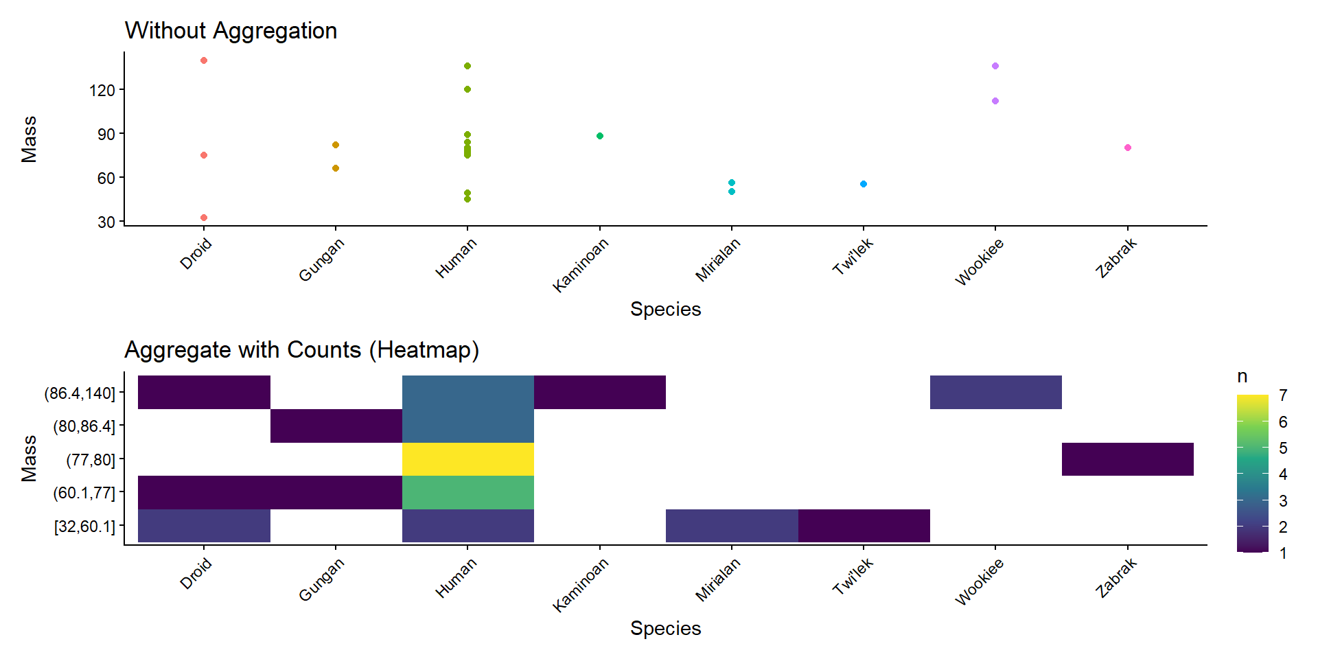

Aggregation

Item Aggregation

2D Summary Stats

# 'sw' created on an earlier slide

a <- sw %>% 
  ggplot(aes(x = height, y = mass)) +
  geom_point(show.legend = FALSE) +
  ggtitle("Without Aggregation") +
  labs(x = "Height", y = "Mass") +
  theme_classic()

b <- sw %>%
  filter(!is.na(mass)) %>% 
  ggplot(aes(x = height, y = mass)) +
  geom_density_2d_filled(show.legend = FALSE) +
  ggtitle("Aggregate with Density (2D KDE)") +
  labs(x = "Height", y = "Mass") +
  scale_fill_viridis_d() +
  theme_classic()

a/b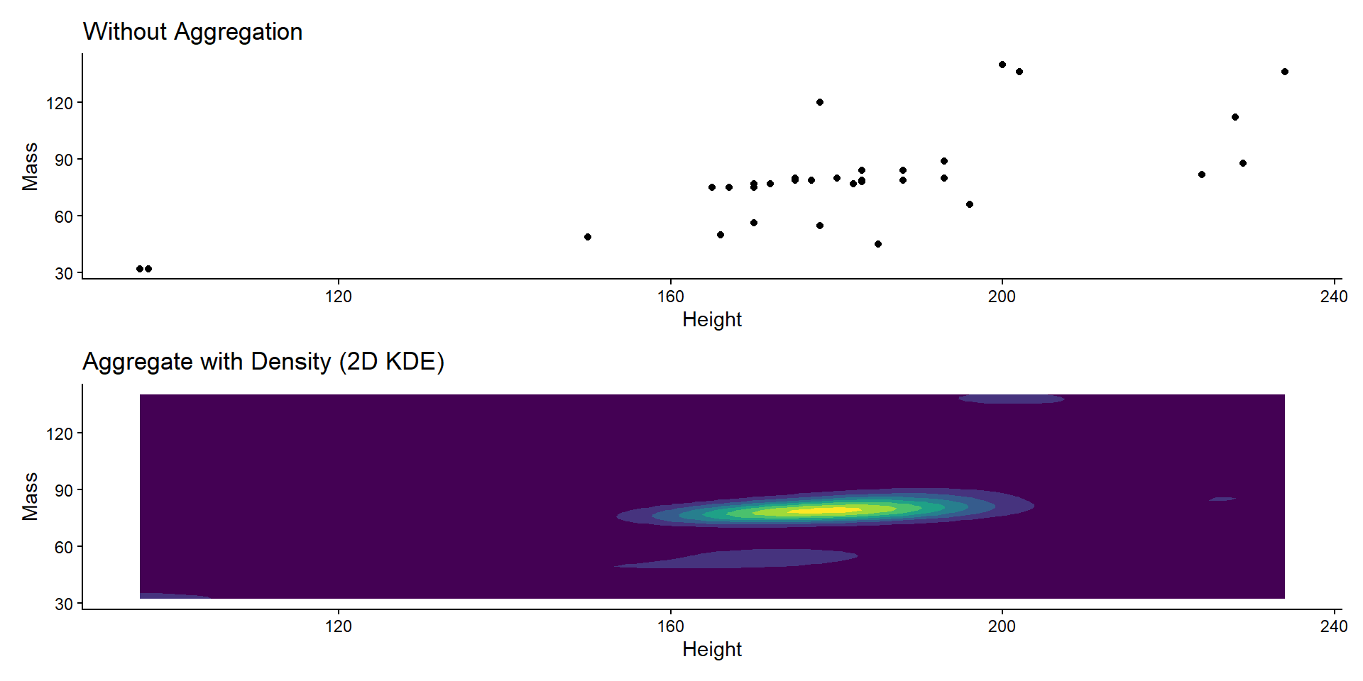

Aggregation

Attribute Aggregation

• Generally refered to as dimensionality reduction (Wikipedia).
• Goal is preserve meaningful structure while using fewer attributes.
• Sometimes, simple solutions exist.
• Mostly involves complex mathematics.

Aggregation

Attribute Aggregation

• Simple solution:

\[BMI = kg/m^2\]

# 'sw' created on previous slide

a <- sw %>% 
  ggplot(aes(x = height, y = mass, color = species)) +
  geom_point() +
  coord_cartesian(xlim = c(50, 250)) +
  ggtitle("Without Aggregation") +
  labs(x = "Height", y = "Mass") +
  theme_classic()

b <- sw %>% 
  mutate(bmi = mass/(height^2)) %>% 
  ggplot(aes(x = species, y = bmi, 
             color = species)) +
  geom_boxplot(show.legend = FALSE) +
  ggtitle("Aggregate with BMI") +
  labs(x = "Species", y = "BMI") +
  theme_classic() +
  theme(axis.text.x = element_text(angle = 45, hjust = 1))

a / b + plot_layout(guides = "collect")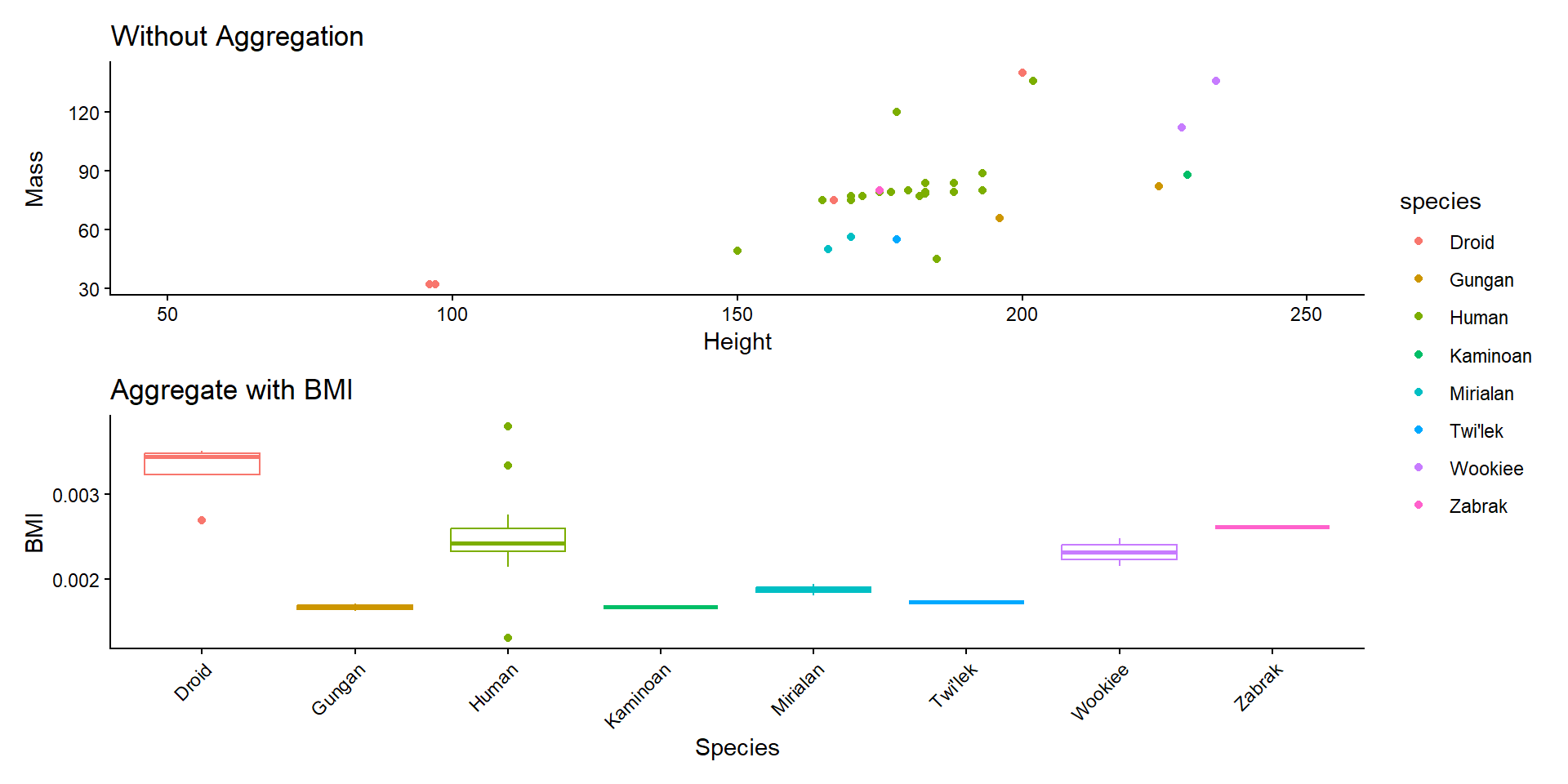

Aggregation

Attribute Aggregation

• Complex methods include:
  • Principal components analysis (PCA)
  • Multidimensional scaling (MDS)
    • Non-metric multidimensional scaling (NMDS)
  • Linear discriminant analysis (LDA)
  • Canonical correlation analysis (CCA)
  • Many others

PCA figure from Wikipedia

Aggregation

Attribute Aggregation

PCA

# 'sw' created earlier; adding BMI here
sw <- sw %>% 
  mutate(bmi = mass/height^2)

pca <- prcomp(~ height + mass, data = sw)
pred <- predict(pca, sw)
sw$pc1 <- pred[, 1]

par(mfrow = c(1, 2))
biplot(pca)
summ <- summary(pca)
barplot(summ$importance[2, ],
        ylim = c(0, 1), ylab = "Proportion",
        main = "Variance Explained")
box()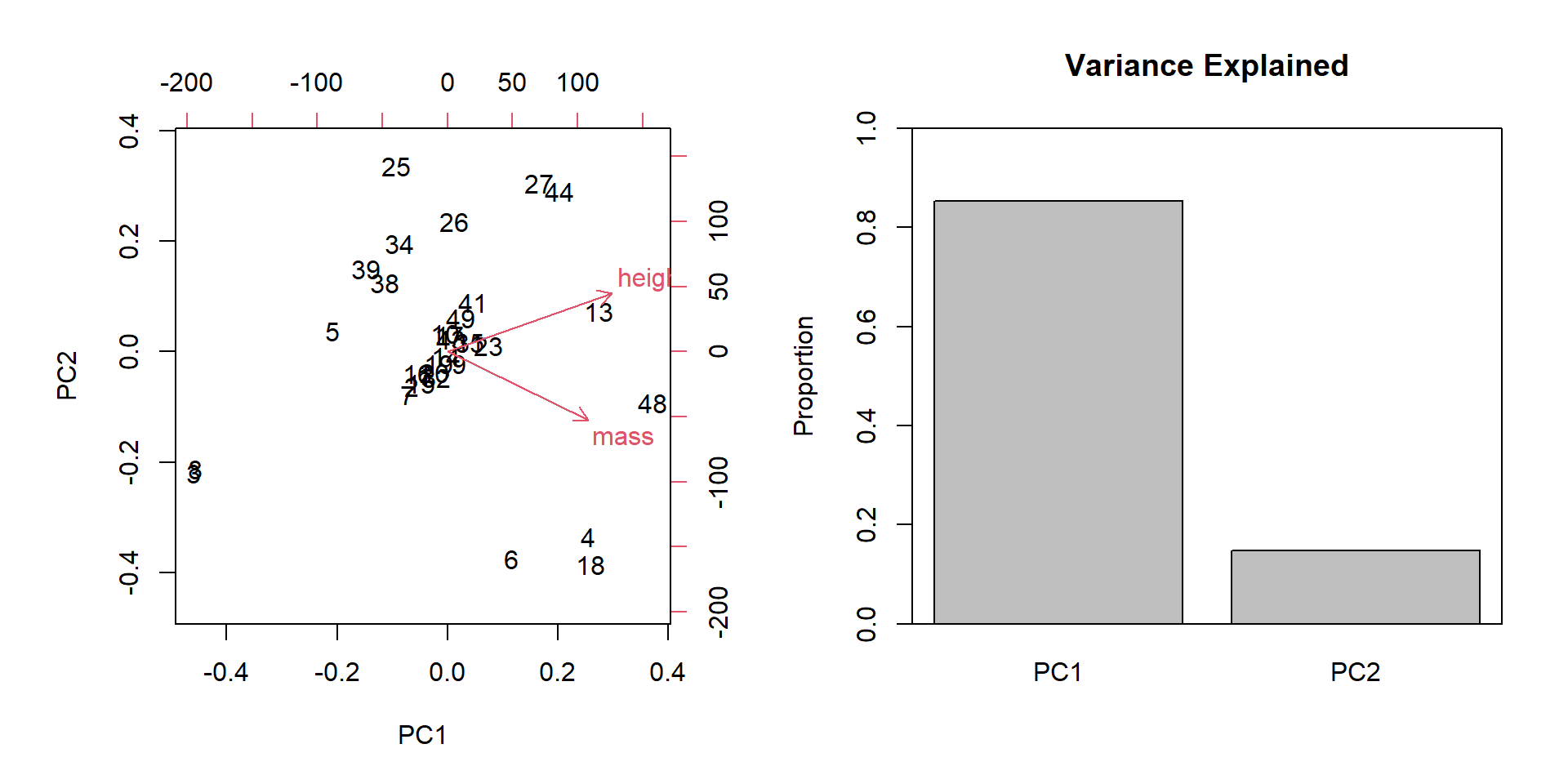

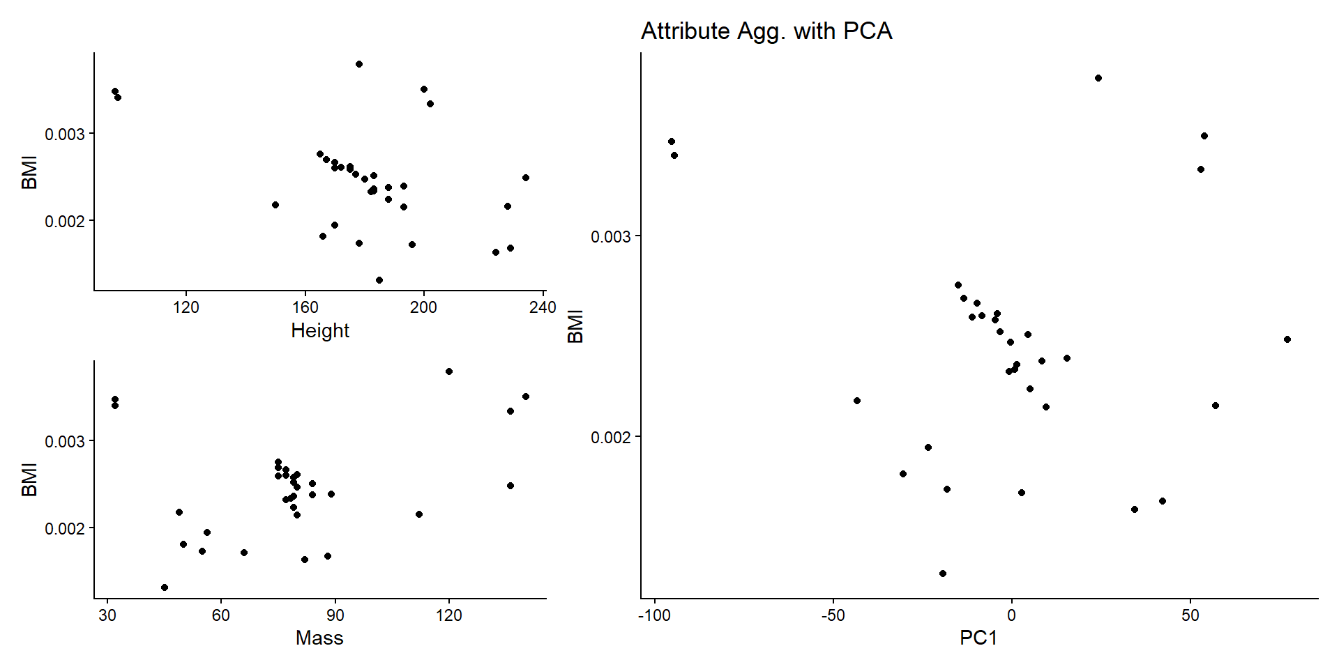
Aggregation

Attribute Aggregation

PCA

# 'sw' created earlier
a <- sw %>% 
  ggplot(aes(x = height, y = bmi)) +
  geom_point() +
  labs(x = "Height", y = "BMI") +
  theme_classic()

b <- sw %>% 
  ggplot(aes(x = mass, y = bmi)) +
  geom_point() +
  labs(x = "Mass", y = "BMI") +
  theme_classic()

c <- sw %>% 
  ggplot(aes(x = pc1, y = bmi)) +
  geom_point() +
  labs(x = "PC1", y = "BMI") +
  ggtitle("Attribute Agg. with PCA") +
  theme_classic()

des <- "AC
        BC"

a + b + c + plot_layout(widths = c(0.4, 0.6),
                        design = des)

Questions?

BCB5200 Home