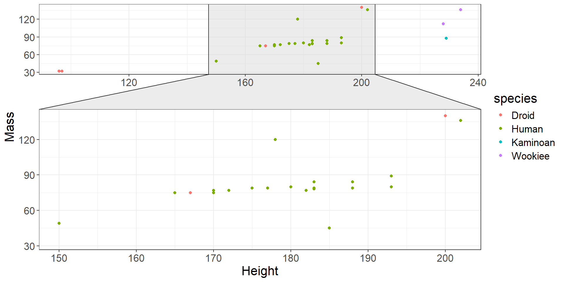
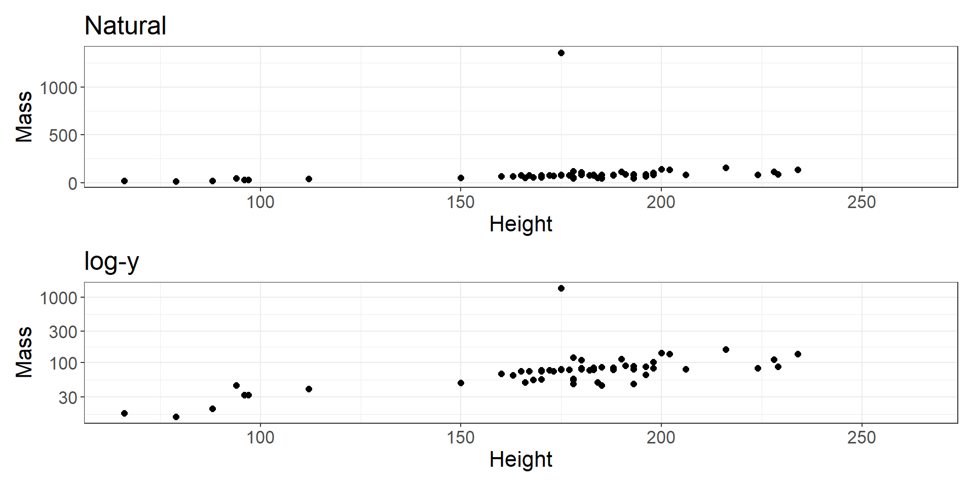
Lecture 15: Embedding

Brian J. Smith

2026-03-31

Reducing Items and Attributes

The beginning of this lecture is based on Chapter 14 of Visualization Analysis & Design.

“Embed: Focus+Context”

For this lecture, I’m going to start with the VAD Text, then transition over to R.

Fig. 14.1

Embed

Why?

• Mitigate possibility of disorientation.
• Support orientation by providing context.
• Reduce cognitive load. (“Eyes beat memory”)

Embed

“Embedding idioms cannot be fully understood when considered purely from the visual encoding point of view or purely from the interaction point of view; they are fundamentally a synthesis of both.”

Embed

How?

• Elide
  • Selectively omit data.
• Superimpose
  • Plot data in layers.
• Distort geometry
  • To emphasize part of the view.

Elide

• With elision, we (1) omit some items from the view completely, (2) summarize other items using aggregation, and (3) show some items in full detail.

library(ggforce)

data("starwars")

starwars %>% 
  filter(species %in% c("Human", "Droid", "Kaminoan", "Wookiee")) %>% 
  ggplot(aes(x = height, y = mass, color = species)) +
  ggforce::facet_zoom(x = species == "Human") +
  geom_point() +
  labs(x = "Height", y = "Mass") +
  theme_bw() +
  theme(text = element_text(size = 16))

Elide

• A general framework for deciding which data to show is the degree of interest (DOI) function.
  • \(DOI = I(x) - D(x, y)\)
    • \(I\) is an interest function. (how much you want to see the item)
    • \(D\) is a distance function. (how far it is from the selected item)
    • \(x\) is the location of the item.
    • \(y\) is the current focus point.
  • Continuous function; often need to choose thresholds for omit/summarize/detail.

Elide

DOI functions

Fig. 1 from Heer and Card (2004)

Heer and Card (2004)

Superimpose

• Add layers to a visualization.
  • Can be global layers showing the entire dataset.
  • Can be local layers showing a zoomed view.

Superimpose

Global

• When units are the same, a single y-axis is not misleading.

url <- 'http://people.whitman.edu/~hundledr/courses/M250F03/LynxHare.txt'
lh <- read.table(url)
names(lh) <- c("year", "hare", "lynx")

lhp <- ggplot(lh, aes(x = year))  +
  geom_line(aes(y = hare, color = "Hare"), linewidth = 1.5) +
  geom_line(aes(y = lynx, color = "Lynx"), linewidth = 1.5) +
  coord_cartesian(ylim = c(0, NA)) +
  scale_color_discrete(name = "Population") +
  xlab("Year") +
  ylab("Population Size (thousands)") +
  ggtitle("Lynx-Hare Data") +
  theme_classic() +
  theme(text = element_text(size = 16))
lhp

Superimpose

Global

• When units differ (or are on a different scale), two y-axes can be misleading.

# Yellowstone northern range elk estimates
elk <- read.csv("data/elk_ssm_estimates_2025.csv") %>% 
  filter(winter %in% 1995:2019) %>% 
  mutate(elk = round(mean)) %>% 
  select(Year = winter, elk)

# Yellowstone northern range (only) wolf abundance
wolf <- read.csv("data/nr_wolf.csv") %>% 
  select(Year = year, wolf = nr_wolf)

# Combine
comb <- elk %>% 
  left_join(wolf, by = "Year")

# Plot on one axis
one_y <- comb %>% 
  pivot_longer(cols = elk:wolf,
               names_to = "Species",
               values_to = "Abundance") %>% 
  ggplot(aes(x = Year, y = Abundance, color = Species)) +
  geom_line(linewidth = 1.5) +
  ggtitle("One y-axis") +
  theme_bw() +
  theme(text = element_text(size = 16))

# Plot on two y-axes
two_y <- comb %>% 
  mutate(wolf = wolf * 200) %>% 
  pivot_longer(cols = elk:wolf,
               names_to = "Species",
               values_to = "Abundance") %>% 
  ggplot(aes(x = Year, y = Abundance, color = Species)) +
  geom_line(linewidth = 1.5) +
  scale_y_continuous(name = "Elk",
                     sec.axis = sec_axis(~ . * 2e-2, name = "Wolves")) +
  coord_cartesian(ylim = c(0, NA)) +
  ggtitle("Two y-axes") +
  theme_bw() +
  theme(text = element_text(size = 16))

# Combine
one_y/two_y + plot_layout(guides = "collect")

Superimpose

Local

• Particularly useful for interactive visualizations.
• Hides the data behind the superimposed layer.

lhp_zoom <- lhp +
  coord_cartesian(xlim = c(1880, 1900)) +
  ggtitle(NULL) +
  xlab(NULL) +
  ylab(NULL) +
  theme(text = element_text(size = 12),
        legend.position = "none",
        plot.background = element_rect(colour = "black", fill = "white", linewidth = 3))

lhp +
  inset_element(lhp_zoom, 0.15, 0.2, 0.85, 0.8)

Superimpose

Local

• See also the package ggmagnify

# install.packages("ggmagnify", repos = c("https://hughjonesd.r-universe.dev", 
#                  "https://cloud.r-project.org"))
# install.packages("ggfx")

library(ggmagnify)
library(ggfx)

# Adapted from ?geom_magnify
ggp <- ggplot(iris, aes(Sepal.Width, Sepal.Length, 
                        color = Species)) +
         geom_point() + 
  xlim(c(2, 6)) +
  theme_bw() +
  theme(text = element_text(size = 16))
from <- list(2.5, 3.5, 6, 7)
to <- list(4, 6, 5, 7)

ggp + 
  geom_magnify(from = from, to = to, 
               shape = "ellipse",
               shadow = TRUE)

Distort

• Geometric distortion can highlight a focal region.
• Important decisions:
  • How many focus regions?
    • 1? More?
  • What shape is the focus?
    • Round? Rectangular? Other?
  • What is the extent of the focus?
    • Global? Local?
  • Will you use interaction? How?
    • E.g., magnifying glass, stretching a rubber sheet, etc.

Distort

• Simplest case of distortion is a nonlinear transformation of the axes.

sw_linear <- starwars %>% 
  ggplot(aes(x = height, y = mass)) +
  geom_point(size = 2) +
  labs(x = "Height", y = "Mass") +
  theme_bw() + 
  ggtitle("Natural") +
  theme(text = element_text(size = 16))

sw_log <- sw_linear +
  scale_y_log10() +
  ggtitle("log-y")

sw_linear/sw_log

Distort

• A popular distortion is the fisheye.
• I found an R Bloggers Post about this, but it doesn’t seem to work well with a scatterplot.
  • R Bloggers Post
    • Here’s a conceptual paper: Keahey (1998)
    • Here’s an interactive example: AntV fisheye
  • It does seem to work well with network/spatial data.
    • Sakar and Brown (1992)
    • Cartograms on the R Graph Gallery

Distort

Costs

• Distance and length judgements are severely impaired.
• Users may be unaware of distortion.
  • Especially without a distorted frame or gridlines.
• Requires cognitive load of object constancy.
  • Remembering an item in two different views is the same item.

Benefits

• Shows the context and the focus in a single view.
• Avoids the need for faceting or reducing.
• Works well with:
  • Familiar shapes (e.g., cartograms)
  • Link-node relationships in networks.

Embedding with R

Elide

• Can be done with faceting.
  • E.g., ggplot2::facet_wrap()
• Can be done with a different view.
  • E.g., patchwork
  • E.g., ggforce::facet_zoom()

Superimpose

• Can be done with multiple axes.
  • E.g., ggplot2::scale_y_continuous(..., sec.axis = sec_axis(...))
• Can be done with an inset panel.
  • E.g., patchwork::inset_element()
  • E.g., ggmagnify::geom_magnify()
  • E.g., ggmapinset::geom_inset_frame() (for maps)

Distort

• Can be done by transforming axes.
  • E.g., ggplot2::coord_transform()
  • I wish it could show untransformed gridlines.
• ggplot2 doesn’t seem very amenable to this, but custom transforms can be done prior to plotting.

Questions?

BCB5200 Home