Lecture 19: Animation
2026-04-21
gganimate
- R package extending
ggplot2for animation.
gganimate README AnimationTransitions
transition_states()- Used to transition using discrete variables (i.e., factors).
- Think of this as an alternative to
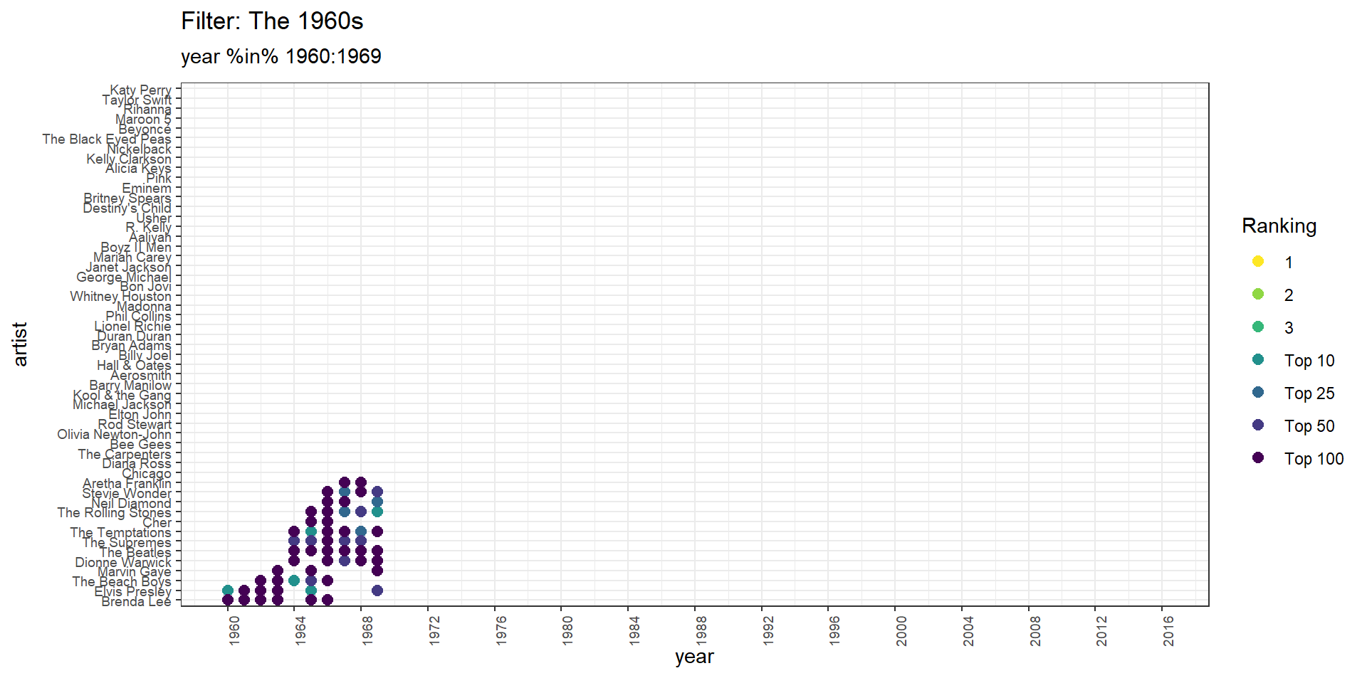
facet_wrap().- E.g., we made this figure in Lecture 12
Transitions
transition_states()- Animate rather than facet:
Transitions
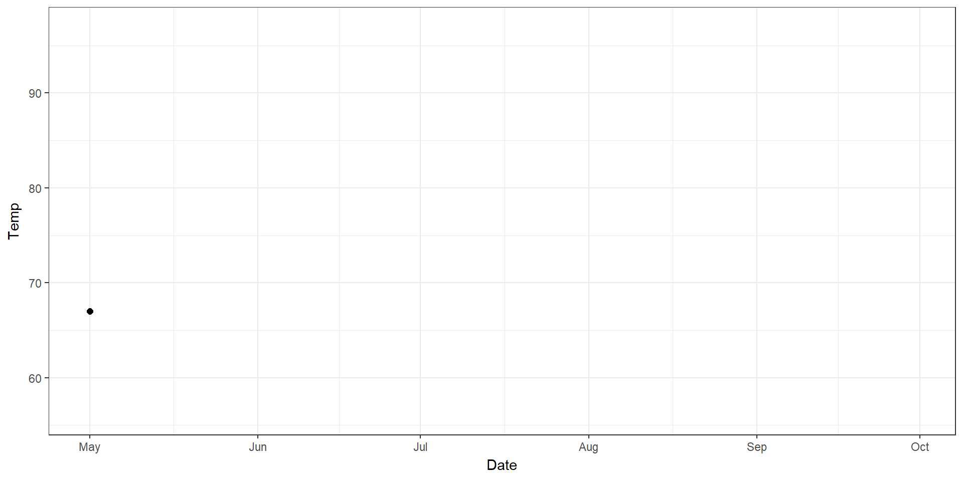
transition_time()- Used to transition using continuous variables (e.g., time).
- An alternative to showing a classic timeseries.
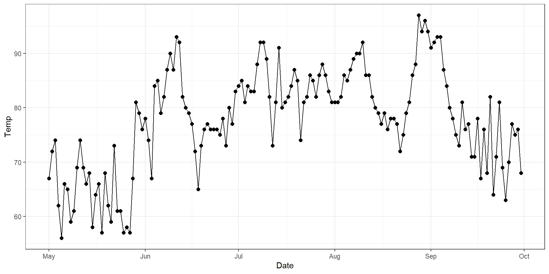
Transitions
transition_time()- (Time shown redundantly with x-position)

Transitions
transition_reveal()- Used to gradually reveal along a dimension.
Transitions
transition_events()- Gives you detailed control over when items enter and exit.
- Static plot:
Code
# Plot
p <- ggplot(tens_fl, aes(x = year, y = artist, color = no_cat)) +
  geom_point(size = 2.5) +
  scale_color_viridis_d(name = "Ranking", direction = -1) +
  scale_x_continuous(breaks = seq(1960, 2016, by = 4)) +
  theme_bw() +
  theme(axis.text.x = element_text(angle = 90, hjust = 1),
        axis.text = element_text(size = 7))
p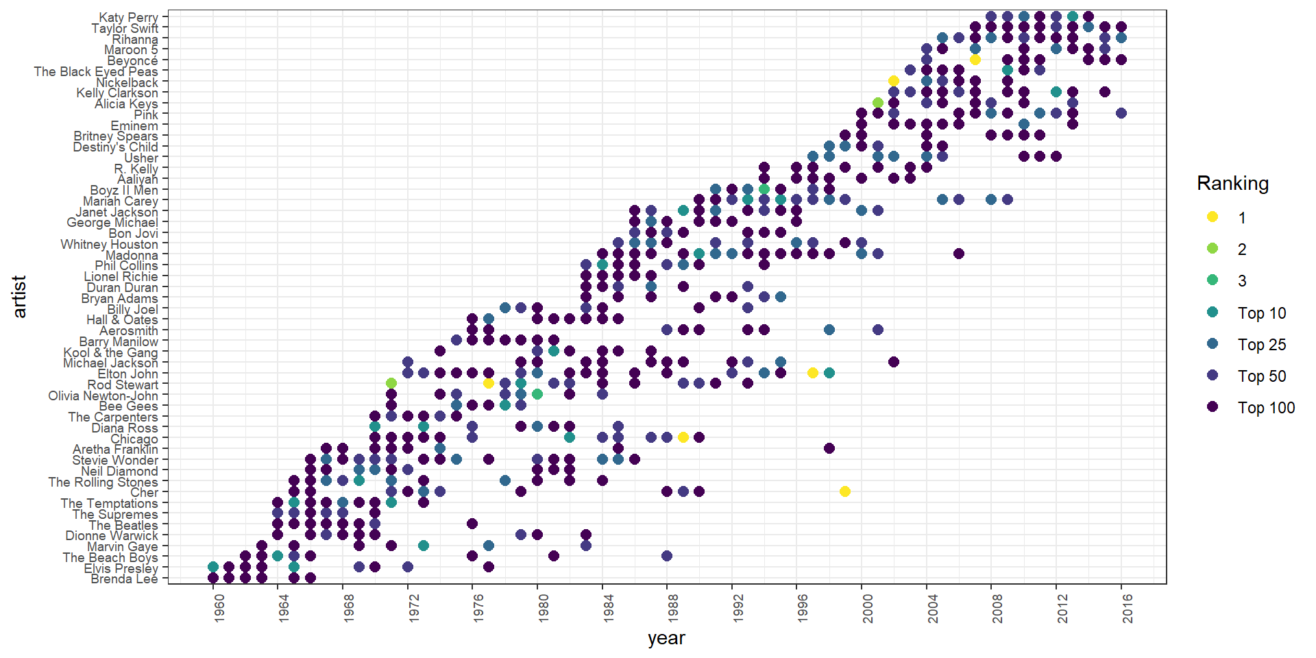
Transitions
transition_events()- Gives you detailed control over when items enter and exit.
- Animation that groups contemporaries together:
Transitions
transition_filter()- Let’s you use sequential filters to remove pieces of data.
- Useful for gradually arriving at a relevant subset of data.
Transition
transition_layers()- Build-up an animation one layer at a time.
- I.e., add each
geomsequentially.
Code
# Plot penguins data
data("penguins")

p <- penguins %>%
  ggplot() +
  geom_point(aes(x = bill_len, y = flipper_len, color = species)) +
  geom_smooth(aes(x = bill_len, y = flipper_len),
              method = "lm", color = "gray30", linetype = "dashed") +
  geom_smooth(aes(x = bill_len, y = flipper_len, color = species),
              method = "lm") +
  coord_cartesian(xlim = c(30, 60),
                  ylim = c(170, 240)) +
  labs(x = "Bill Length (mm)",
       y = "Flipper Length (mm)") +
  theme_bw()

p 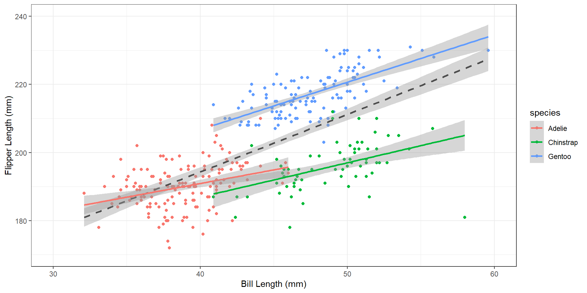
Transition
transition_layers()- Build-up an animation one layer at a time.
- I.e., add each
geomsequentially.
Transition
transition_components()- Transitions individual “components” around the figure.
- Each component has its own time column, so can enter and exit at any time.
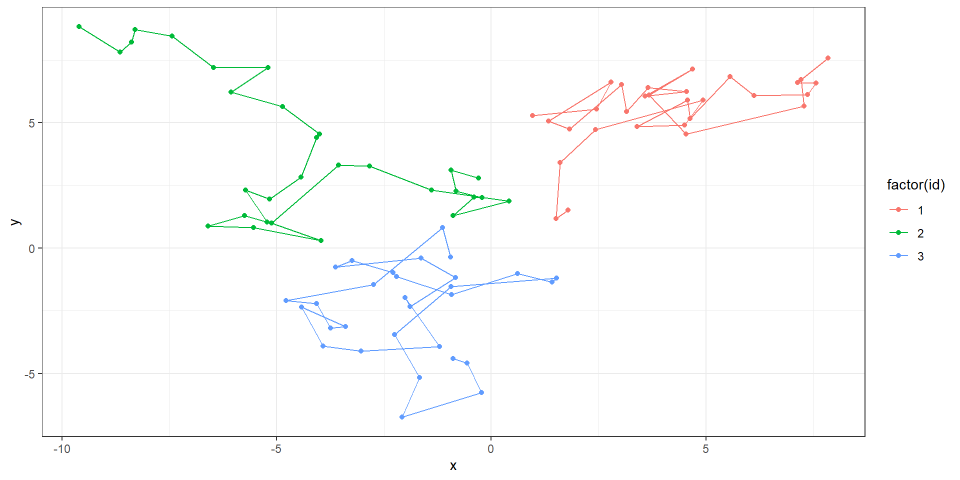
Transition
transition_components()- Transitions individual “components” around the figure.
- Each component has its own time column, so can enter and exit at any time.
Code
dat %>%
  # Let ID 1 go all 30 timesteps
  # Only let ID 2 enter at t = 10
  # Have ID 3 go from t = 5 to 20
  filter(id == 1 | (id == 2 & t > 9) | (id == 3 & t %in% 5:20)) %>%
  ggplot(aes(x = x, y = y, color = factor(id), group = factor(id))) +
  geom_point(size = 3) +
  theme_bw() +
  transition_components(time = t) +
  ggtitle("t = {frame_time}")
Views
view_follow()- Follow the data in each frame.
Code
penguins %>%
  filter(!is.na(bill_len),
         !is.na(flipper_len)) %>%
  ggplot(aes(bill_len, flipper_len, color = species)) +
  geom_point() +
  theme_bw() +
  labs(x = "Bill Length (mm)",
       y = "Flipper Length (mm)",
       title = "{closest_state}") +
  transition_states(species, transition_length = 4, state_length = 1) +
  view_follow()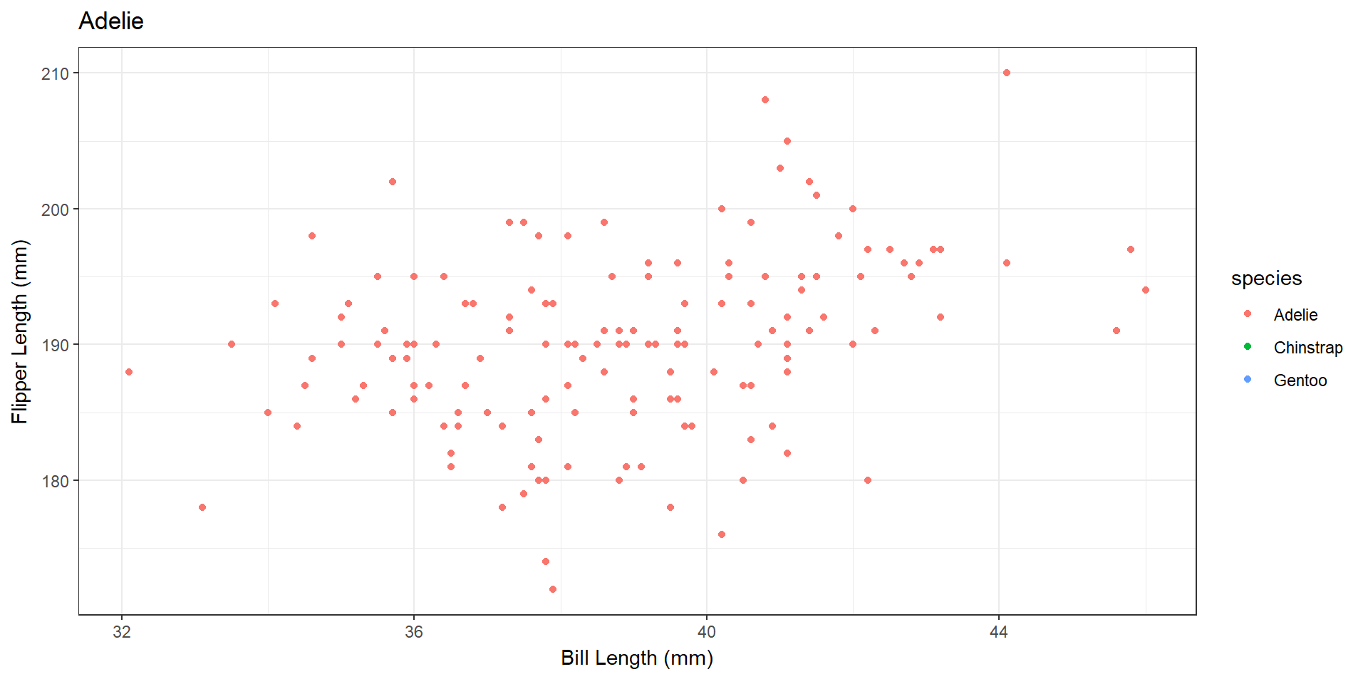
Views
view_step()- Follow the data in steps.
Code
penguins %>%
  filter(!is.na(bill_len),
         !is.na(flipper_len)) %>%
  ggplot(aes(bill_len, flipper_len, color = species)) +
  geom_point() +
  theme_bw() +
  labs(x = "Bill Length (mm)",
       y = "Flipper Length (mm)",
       title = "{closest_state}") +
  transition_states(species, transition_length = 4, state_length = 1) +
  view_step(pause_length = 2, step_length = 1, nsteps = 3)
Views
view_zoom()- Zoom between states.
- Does a combination of zooming and panning.
- Controlled by argument
pan_zoom.
- Controlled by argument
Code
penguins %>%
  filter(!is.na(bill_len),
         !is.na(flipper_len)) %>%
  ggplot(aes(bill_len, flipper_len, color = species)) +
  geom_point() +
  theme_bw() +
  labs(x = "Bill Length (mm)",
       y = "Flipper Length (mm)",
       title = "{closest_state}") +
  transition_states(species, transition_length = 4, state_length = 1) +
  view_zoom(pause_length = 1, step_length = 2, nsteps = 3)
Shadows
shadow_wake()- Show preceding frames with gradual falloff.
Code
penguins %>%
  filter(!is.na(bill_len),
         !is.na(flipper_len)) %>%
  ggplot(aes(bill_len, flipper_len, color = species)) +
  geom_point() +
  theme_bw() +
  labs(x = "Bill Length (mm)",
       y = "Flipper Length (mm)",
       title = "{closest_state}") +
  transition_states(species, transition_length = 4, state_length = 1) +
  shadow_wake(wake_length = 0.1)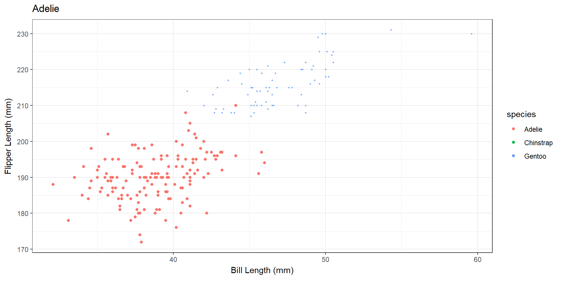
Shadows
shadow_trail()- A trail of evenly spaced old frames.
Code
dat %>%
  # Let ID 1 go all 30 timesteps
  # Only let ID 2 enter at t = 10
  # Have ID 3 go from t = 5 to 20
  filter(id == 1 | (id == 2 & t > 9) | (id == 3 & t %in% 5:20)) %>%
  ggplot(aes(x = x, y = y, color = factor(id), group = factor(id))) +
  geom_point(size = 3) +
  theme_bw() +
  transition_components(time = t) +
  ggtitle("t = {frame_time}") +
  shadow_trail(max_frames = 3, alpha = 0.3)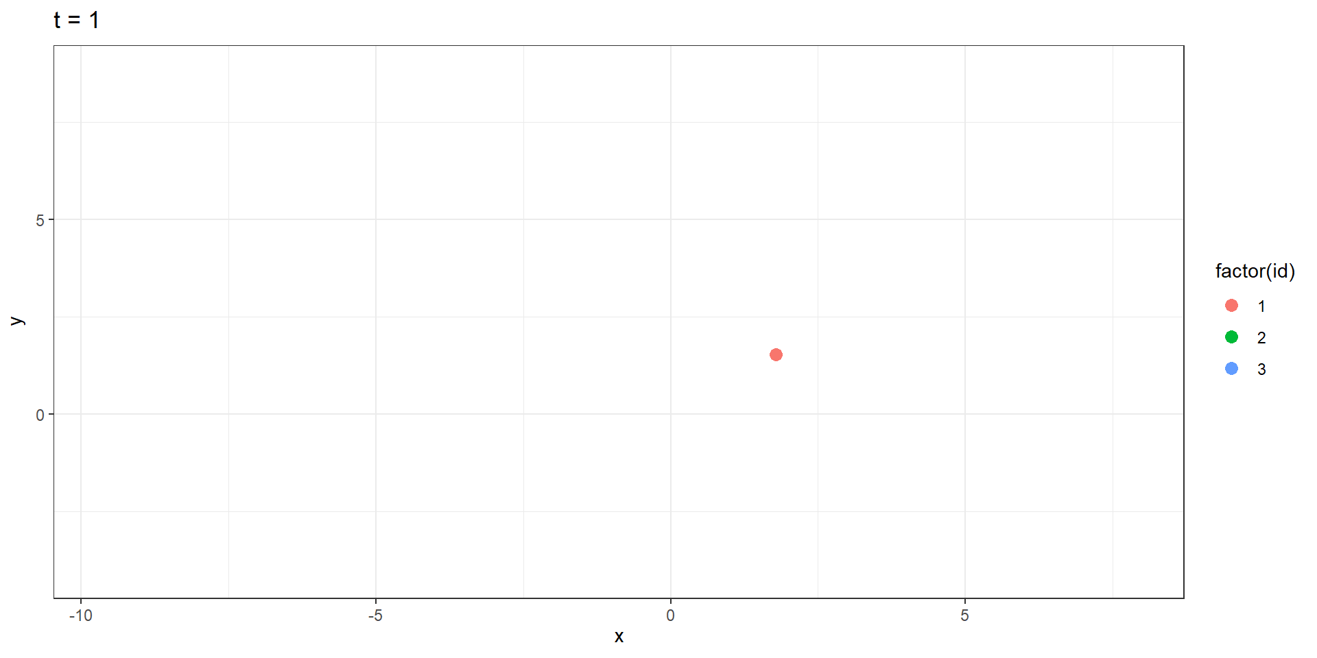
Shadows
shadow_mark()- Show original data as background marks.
Code
penguins %>%
  filter(!is.na(bill_len),
         !is.na(flipper_len)) %>%
  ggplot(aes(bill_len, flipper_len, color = species)) +
  geom_point() +
  theme_bw() +
  labs(x = "Bill Length (mm)",
       y = "Flipper Length (mm)",
       title = "{closest_state}") +
  transition_states(species, transition_length = 1, state_length = 1) +
  shadow_mark(past = TRUE, future = TRUE, colour = 'grey')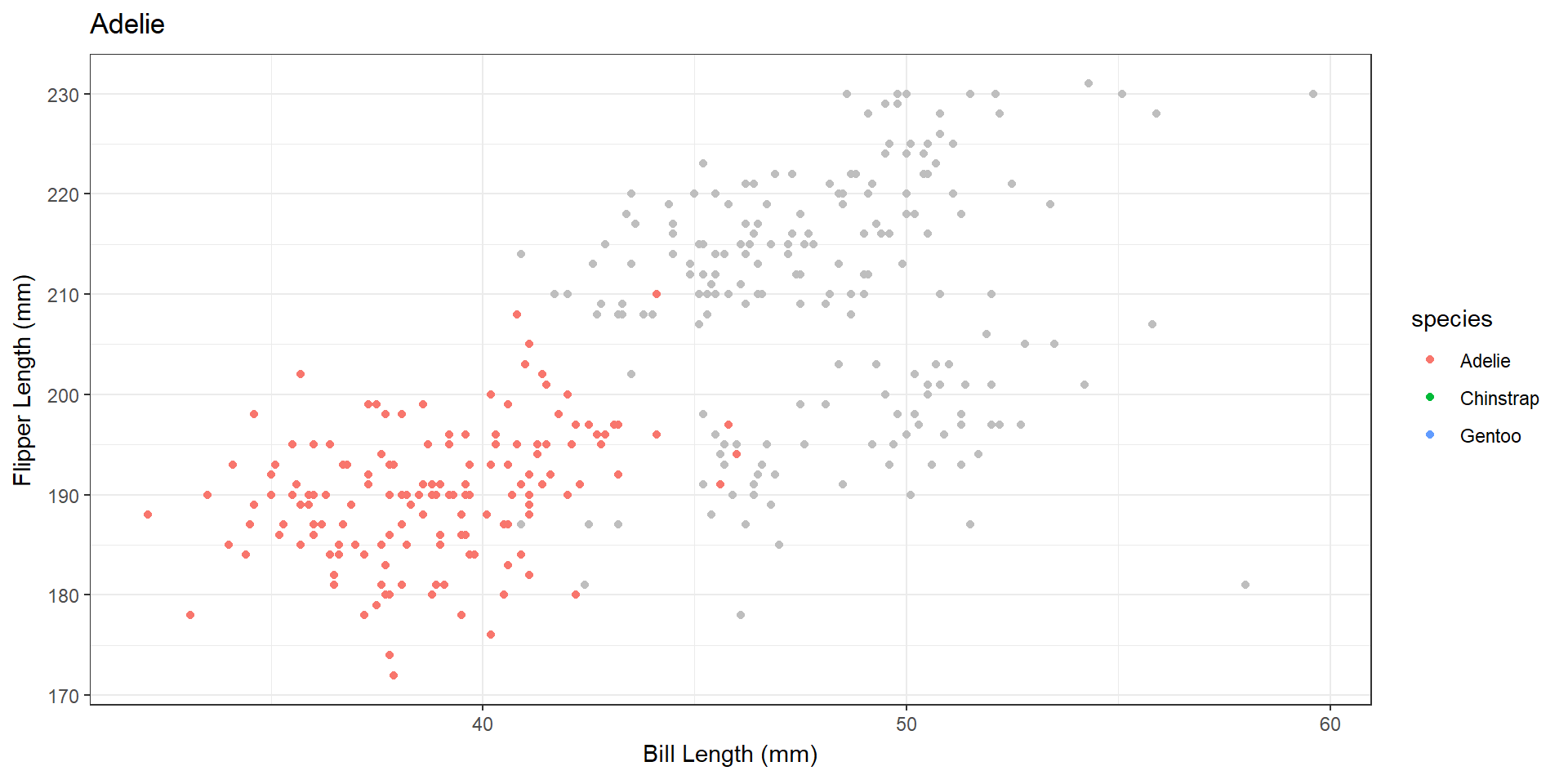
Tweening
enter_appear()/exit_disappear()- Default options for transitions.
Code
penguins %>%
  filter(!is.na(bill_len),
         !is.na(flipper_len)) %>%
  ggplot(aes(bill_len, flipper_len, color = species)) +
  geom_point() +
  theme_bw() +
  labs(x = "Bill Length (mm)",
       y = "Flipper Length (mm)",
       title = "{closest_state}") +
  transition_states(species, transition_length = 1, state_length = 1) +
  enter_appear() +
  exit_disappear()
Tweening
enter_fade()/exit_fade()
Code
penguins %>%
  filter(!is.na(bill_len),
         !is.na(flipper_len)) %>%
  ggplot(aes(bill_len, flipper_len, color = species)) +
  geom_point() +
  theme_bw() +
  labs(x = "Bill Length (mm)",
       y = "Flipper Length (mm)",
       title = "{closest_state}") +
  transition_states(species, transition_length = 1, state_length = 1) +
  enter_fade() +
  exit_fade()
Tweening
enter_grow()/exit_shrink()
Code
penguins %>%
  filter(!is.na(bill_len),
         !is.na(flipper_len)) %>%
  ggplot(aes(bill_len, flipper_len, color = species)) +
  geom_point() +
  theme_bw() +
  labs(x = "Bill Length (mm)",
       y = "Flipper Length (mm)",
       title = "{closest_state}") +
  transition_states(species, transition_length = 3, state_length = 1) +
  enter_grow() +
  exit_shrink()
Tweening
enter_recolor()/exit_recolor()
Code
penguins %>%
  filter(!is.na(bill_len),
         !is.na(flipper_len)) %>%
  ggplot(aes(bill_len, flipper_len, color = species)) +
  geom_point() +
  theme_bw() +
  labs(x = "Bill Length (mm)",
       y = "Flipper Length (mm)",
       title = "{closest_state}") +
  transition_states(species, transition_length = 2, state_length = 1) +
  enter_recolor(color = "gray") +
  exit_recolor(color = "gray")
Tweening
enter_fly()/exit_fly()
Code
penguins %>%
  filter(!is.na(bill_len),
         !is.na(flipper_len)) %>%
  ggplot(aes(bill_len, flipper_len, color = species)) +
  geom_point() +
  theme_bw() +
  labs(x = "Bill Length (mm)",
       y = "Flipper Length (mm)",
       title = "{closest_state}") +
  transition_states(species, transition_length = 1, state_length = 1) +
  enter_fly(x_loc = 30, y_loc = 170) +
  exit_fly(x_loc = 60, y_loc = 230)
Tweening
enter_drift()/exit_drift()
Code
penguins %>%
  filter(!is.na(bill_len),
         !is.na(flipper_len)) %>%
  ggplot(aes(bill_len, flipper_len, color = species)) +
  geom_point() +
  theme_bw() +
  labs(x = "Bill Length (mm)",
       y = "Flipper Length (mm)",
       title = "{closest_state}") +
  transition_states(species, transition_length = 1, state_length = 1) +
  enter_drift(x_mod = 20) +
  exit_drift(y_mod = 100)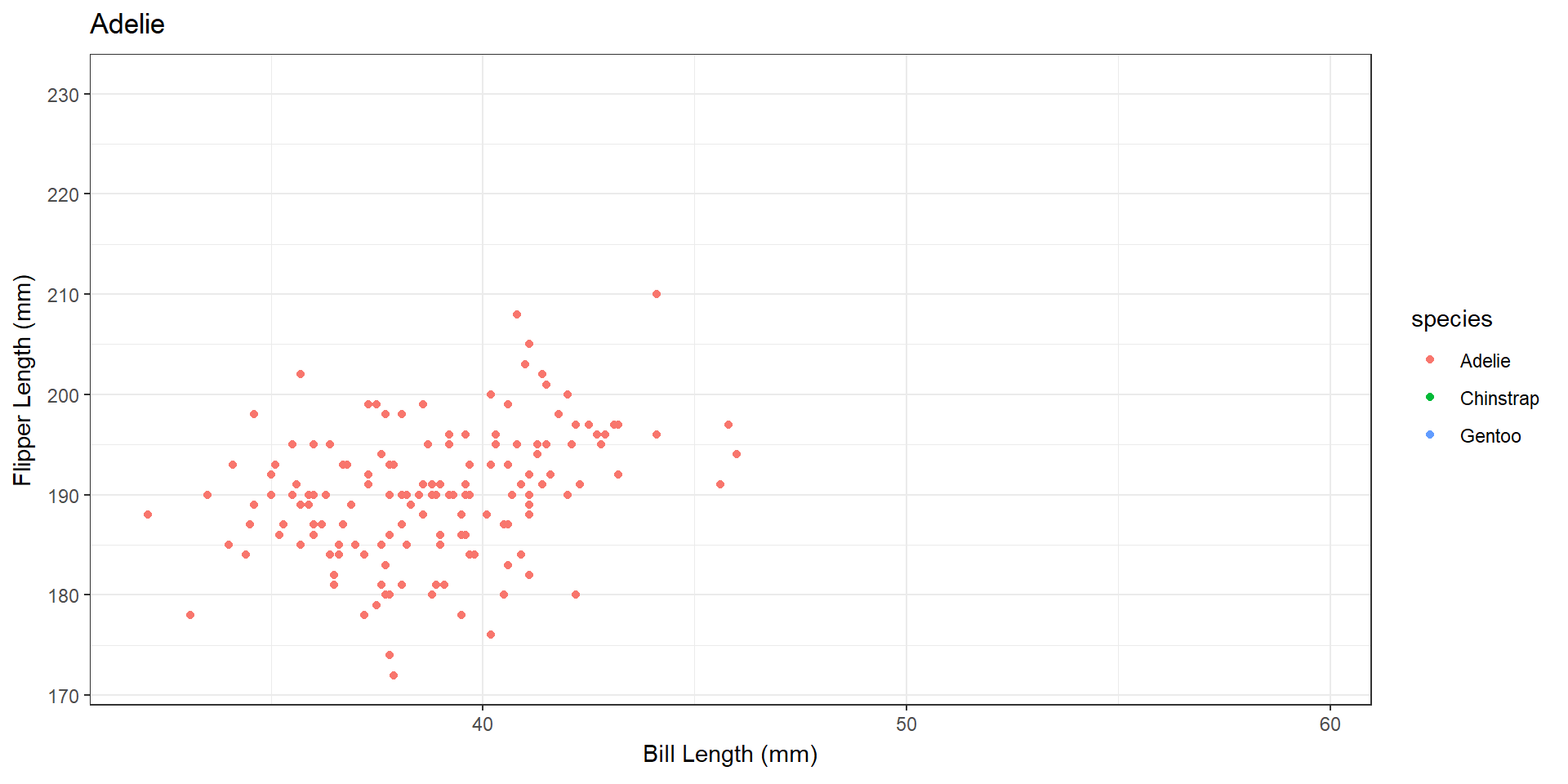
Tweening
- You can combine multiple
enter_*()/exit_*()effects.
Code
penguins %>%
  filter(!is.na(bill_len),
         !is.na(flipper_len)) %>%
  ggplot(aes(bill_len, flipper_len, color = species)) +
  geom_point() +
  theme_bw() +
  labs(x = "Bill Length (mm)",
       y = "Flipper Length (mm)",
       title = "{closest_state}") +
  transition_states(species, transition_length = 2, state_length = 1) +
  # Two enter_*()
  enter_fade() + enter_grow() +
  # Two exit_*()
  exit_fly(x_loc = 7, y_loc = 40) + exit_recolor(color = "black")
Custom Animations